ggchangepoint

One interface. 31 changepoint methods. Every result tidy, every result plottable.

ggchangepoint wraps the R changepoint ecosystem behind a single tidy, ggplot2-native interface: cpt_detect() runs any of 31 detection methods, every result comes back as the same tidy ggcpt object, and autoplot() draws it.

Installation

Install the released version from CRAN:

install.packages("ggchangepoint")

Or the development version from GitHub:

# install.packages("devtools")
devtools::install_github("PursuitOfDataScience/ggchangepoint")

Quick start

library(ggchangepoint)
library(ggplot2)

Generate a series with a mean shift:

set.seed(2022)
x <- c(rnorm(100, 0, 1), rnorm(100, 10, 1))

Detect changepoints with the unified cpt_detect():

res <- cpt_detect(x, method = "pelt", change_in = "mean")
res
#> ggcpt (changepoint detection result)
#>   Method:          pelt 
#>   Change in:       mean 
#>   Changepoints found: 1 
#>   CP convention:   left 
#>   Penalty:         MBIC = NA 
#>   Series length:   200 
#> 
#> Changepoints:
#> # A tibble: 1 × 2
#>      cp cp_value
#>   <int>    <dbl>
#> 1   100    0.467

The result is a ggcpt S3 object. Print it to see the changepoints, or use tidy(), glance(), and augment():

tidy(res)
#> # A tibble: 1 × 2
#>      cp cp_value
#>   <int>    <dbl>
#> 1   100    0.467
glance(res)
#> # A tibble: 1 × 9
#>       n n_changepoints method change_in penalty_type penalty_value cp_convention
#>   <int>          <int> <chr>  <chr>     <chr>                <dbl> <chr>        
#> 1   200              1 pelt   mean      MBIC                    NA left         
#> # ℹ 2 more variables: total_cost <dbl>, runtime <dbl>

Visualise with autoplot():

autoplot(res)

Why ggchangepoint

• Detect with one call — cpt_detect(x, method = "...") dispatches to 31 methods, from classic PELT to Bayesian online detection.
• Tidy everywhere — every method returns the same ggcpt object, with tidy(), glance(), and augment().
• Plot everything — autoplot() draws any result: changepoints, confidence intervals, fitted signals, posteriors, multivariate facets.
• Trust the answer — compare methods side by side, sweep the penalty (CROPS), bootstrap stability, and score accuracy against ground truth.

Family	Methods
Penalised / optimal	PELT · BinSeg · SegNeigh · AMOC · FPOP · CROPS path · fastcpd (ARMA/GARCH) · CPOP (slope)
Multiscale / search	WBS · WBS2 · TGUH · NOT · MOSUM · Isolate-Detect · SMUCE/HSMUCE (with CIs)
Nonparametric / kernel	ED-PELT · E-Divisive · E-Agglo · kernel running stats · NP-MOJO · CPM · self-normalisation
Bayesian	bcp posteriors · online BOCPD · BEAST model averaging
Multivariate / regression	inspect · ocd · geomcp · Bai–Perron · segmented · EnvCpt · DeCAFS

Run cpt_methods() for the live table with engines and installation status. Only changepoint, changepoint.np, and ecp are required — every other engine is optional (Suggests), and the original 0.1.0 functions (cpt_wrapper(), ecp_wrapper(), ggcptplot(), ggecpplot()) keep working unchanged.

Unified detection across engines

cpt_detect() dispatches to any supported method by name:

cpt_detect(x, method = "binseg", change_in = "mean")
#> ggcpt (changepoint detection result)
#>   Method:          binseg 
#>   Change in:       mean 
#>   Changepoints found: 1 
#>   CP convention:   left 
#>   Penalty:         MBIC = NA 
#>   Series length:   200 
#> 
#> Changepoints:
#> # A tibble: 1 × 2
#>      cp cp_value
#>   <int>    <dbl>
#> 1   100    0.467
cpt_detect(x, method = "wbs", change_in = "mean")
#> ggcpt (changepoint detection result)
#>   Method:          wbs 
#>   Change in:       mean 
#>   Changepoints found: 1 
#>   CP convention:   left 
#>   Penalty:         sSIC = NA 
#>   Series length:   200 
#> 
#> Changepoints:
#> # A tibble: 1 × 2
#>      cp cp_value
#>   <int>    <dbl>
#> 1   100    0.467
cpt_detect(x, method = "fpop", change_in = "mean")
#> ggcpt (changepoint detection result)
#>   Method:          fpop 
#>   Change in:       mean 
#>   Changepoints found: 1 
#>   CP convention:   left 
#>   Penalty:         Manual = 17.8459510605346 
#>   Series length:   200 
#> 
#> Changepoints:
#> # A tibble: 1 × 2
#>      cp cp_value
#>   <int>    <dbl>
#> 1   100    0.467

Use cpt_methods() to see all available and planned methods with their engine packages and installation status:

cpt_methods()
#> # A tibble: 35 × 6
#>    method   change_in                   engine   status target_release installed
#>    <chr>    <chr>                       <chr>    <chr>  <chr>          <lgl>    
#>  1 pelt     mean, var, meanvar          changep… avail… <NA>           TRUE     
#>  2 binseg   mean, var, meanvar          changep… avail… <NA>           TRUE     
#>  3 segneigh mean, var, meanvar          changep… avail… <NA>           TRUE     
#>  4 amoc     mean, var, meanvar          changep… avail… <NA>           TRUE     
#>  5 np       distribution                changep… avail… <NA>           TRUE     
#>  6 ecp      distribution (multivariate) ecp      avail… <NA>           TRUE     
#>  7 fpop     mean                        fpop     avail… <NA>           TRUE     
#>  8 wbs      mean                        wbs      avail… <NA>           TRUE     
#>  9 wbs2     mean                        breakfa… avail… <NA>           TRUE     
#> 10 not      mean, var, slope            not      avail… <NA>           TRUE     
#> # ℹ 25 more rows

Detection with uncertainty: confidence intervals and posteriors

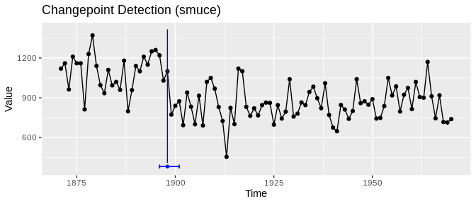
SMUCE (smuce_wrapper(), via stepR) delivers a confidence interval for every changepoint location; Bai–Perron (strucchange_wrapper()) and broken-line regression (segmented_wrapper()) do the same for regression breaks. The intervals live in ci_lower/ci_upper columns and render with autoplot(show_ci = TRUE) or the geom_cpt_ci() layer:

res_smuce <- smuce_wrapper(x)
tidy(res_smuce)
#> # A tibble: 2 × 4
#>      cp cp_value ci_lower ci_upper
#>   <int>    <dbl>    <int>    <int>
#> 1     7   -1.06         2       94
#> 2   100    0.467      100      100
autoplot(res_smuce, show_ci = TRUE, show_fit = TRUE)

Bayesian engines return posterior probabilities instead: bcp_wrapper() (posterior probability of a change at every location), beast_wrapper() (Bayesian model averaging), and bocpd_wrapper() (online run-length posterior). Two dedicated displays accompany them — ggcpt_posterior() and ggcpt_runlength():

res_bcp <- bcp_wrapper(x, seed = 1)
tidy(res_bcp)
#> # A tibble: 1 × 3
#>      cp cp_value posterior_prob
#>   <int>    <dbl>          <dbl>
#> 1   100    0.467              1
ggcpt_posterior(res_bcp)

The penalty path: CROPS

Instead of guessing one penalty, cpt_crops() computes every optimal segmentation over a penalty range (Haynes, Eckley and Fearnhead, 2017) and plots the elbow diagnostic, the penalty path, or the candidate segmentations themselves:

path <- cpt_crops(c(rnorm(100), rnorm(100, 3), rnorm(100, -1)))
path
#> ggcpt_path (CROPS penalty path)
#>   Change in:       mean 
#>   Penalty range:  [5.704, 57.04]
#>   Series length:   300 
#>   Distinct segmentations: 2 
#> 
#> # A tibble: 2 × 3
#>   penalty n_cpts  cost
#>     <dbl>  <int> <dbl>
#> 1    7.68      2  274.
#> 2    5.70      4  259.
autoplot(path)                          # cost elbow

autoplot(path, type = "segmentations")  # see the actual candidate models

Compare methods

ggcpt_compare(x, methods = c("pelt", "binseg", "fpop", "wbs"))

For a numeric summary, use ggcpt_compare_table():

ggcpt_compare_table(x, methods = c("pelt", "binseg", "fpop", "wbs"))
#> # A tibble: 4 × 3
#>   method    cp cp_value
#>   <chr>  <int>    <dbl>
#> 1 pelt     100    0.467
#> 2 binseg   100    0.467
#> 3 fpop     100    0.467
#> 4 wbs      100    0.467

Batch detection and stability diagnostics

cpt_batch() runs one detector over many series (a matrix, data frame, or list) and returns a tidy tibble of results — honouring future::plan() for parallel execution. cpt_stability() bootstrap-resamples within fitted segments and reports how often each location is re-detected, a cheap confidence signal for engines with no native intervals:

X <- cbind(shifted = x, noise = rnorm(200))
batch <- cpt_batch(X, method = "pelt")
batch
#> ggcpt_batch (2 series, method: pelt)
#> 
#> # A tibble: 2 × 2
#>   series  n_changepoints
#>   <chr>            <int>
#> 1 shifted              1
#> 2 noise                0
autoplot(batch)

st <- cpt_stability(x, method = "pelt", B = 50, seed = 1)
st
#> ggcpt_stability (50 bootstrap replicates, method: pelt)
#> 
#> Original changepoints and their re-detection frequency:
#> # A tibble: 1 × 2
#>      cp stability
#>   <int>     <dbl>
#> 1   100         1
autoplot(st)

Multivariate and high-dimensional detection

The multivariate engines accept a matrix (rows are time points) directly through cpt_detect() and render as faceted small-multiples:

set.seed(1)
Xhd <- cbind(a = c(rnorm(80), rnorm(80, 3)),
             b = c(rnorm(80), rnorm(80, -2)),
             c = rnorm(160))
res_hd <- inspect_wrapper(Xhd)
tidy(res_hd)
#> # A tibble: 1 × 3
#>      cp cp_value strength
#>   <int>    <dbl>    <dbl>
#> 1    80   -0.590     21.9
autoplot(res_hd)

Evaluation

When ground truth changepoints are known, compute accuracy metrics (precision/recall/F1 under one-to-one matching, the covering metric, Hausdorff distance, adjusted Rand index):

cpt_metrics(pred = c(100), truth = c(100), n = 200)
#> # A tibble: 1 × 12
#>       n n_pred n_truth precision recall    f1 covering hausdorff rand_index
#>   <int>  <int>   <int>     <dbl>  <dbl> <dbl>    <dbl>     <dbl>      <dbl>
#> 1   200      1       1         1      1     1        1         0          1
#> # ℹ 3 more variables: annotation_error <int>, mae_matched <dbl>,
#> #   rmse_matched <dbl>

When multiple annotation sets are available, use cpt_metrics_annotated(), and visualise agreement with ggcpt_eval():

cpt_metrics_annotated(c(100), list(c(100), c(101), c(99)), n = 200, margin = 5)
#> # A tibble: 1 × 7
#>       n n_annotators n_pred precision recall    f1 covering
#>   <dbl>        <int>  <int>     <dbl>  <dbl> <dbl>    <dbl>
#> 1   200            3      1         1      1     1    0.993

Data simulation

dat <- cpt_simulate(200, changepoints = c(100), change_in = "mean",
                    params = c(0, 10), sd = 1)
attributes(dat)$true_changepoints
#> [1] 100

An alias rcpt() is provided for compatibility. Built-in test signals include signal_blocks() (the Donoho–Johnstone blocks signal), signal_fms(), signal_mix(), signal_teeth(), and signal_stairs().

Penalty configuration

Use cpt_penalty() to construct penalty values for use with detection methods:

cpt_penalty("BIC", n = 200)
#> [1] 5.298317
cpt_penalty("AIC", n = 200)
#> [1] 2
cpt_penalty("Manual", value = 10)
#> [1] 10

Direct engine wrappers

For fine-grained control, every engine has its own wrapper returning a ggcpt object directly. The classic search/pruning engines:

fpop_wrapper(x, penalty = 2 * log(200))
#> ggcpt (changepoint detection result)
#>   Method:          fpop 
#>   Change in:       mean 
#>   Changepoints found: 1 
#>   CP convention:   left 
#>   Penalty:         Manual = 10.5966347330961 
#>   Series length:   200 
#> 
#> Changepoints:
#> # A tibble: 1 × 2
#>      cp cp_value
#>   <int>    <dbl>
#> 1   100    0.467
wbs_wrapper(x, n_intervals = 2000)
#> ggcpt (changepoint detection result)
#>   Method:          wbs 
#>   Change in:       mean 
#>   Changepoints found: 1 
#>   CP convention:   left 
#>   Penalty:         sSIC = NA 
#>   Series length:   200 
#> 
#> Changepoints:
#> # A tibble: 1 × 2
#>      cp cp_value
#>   <int>    <dbl>
#> 1   100    0.467
wbs2_wrapper(x)
#> ggcpt (changepoint detection result)
#>   Method:          wbs2 
#>   Change in:       mean 
#>   Changepoints found: 1 
#>   CP convention:   left 
#>   Penalty:         SDLL = NA 
#>   Series length:   200 
#> 
#> Changepoints:
#> # A tibble: 1 × 2
#>      cp cp_value
#>   <int>    <dbl>
#> 1   100    0.467
not_wrapper(x, contrast = "pcwsConstMean")
#> ggcpt (changepoint detection result)
#>   Method:          not 
#>   Change in:       mean 
#>   Changepoints found: 1 
#>   CP convention:   left 
#>   Penalty:         sSIC = NA 
#>   Series length:   200 
#> 
#> Changepoints:
#> # A tibble: 1 × 2
#>      cp cp_value
#>   <int>    <dbl>
#> 1   100    0.467
mosum_wrapper(x)
#> ggcpt (changepoint detection result)
#>   Method:          mosum 
#>   Change in:       mean 
#>   Changepoints found: 1 
#>   CP convention:   left 
#>   Penalty:         threshold = 3.63416800924526 
#>   Series length:   200 
#> 
#> Changepoints:
#> # A tibble: 1 × 2
#>      cp cp_value
#>   <int>    <dbl>
#> 1   100    0.467
idetect_wrapper(x)
#> ggcpt (changepoint detection result)
#>   Method:          idetect 
#>   Change in:       mean 
#>   Changepoints found: 1 
#>   CP convention:   left 
#>   Penalty:         threshold = NA 
#>   Series length:   200 
#> 
#> Changepoints:
#> # A tibble: 1 × 2
#>      cp cp_value
#>   <int>    <dbl>
#> 1   100    0.467
tguh_wrapper(x)
#> ggcpt (changepoint detection result)
#>   Method:          tguh 
#>   Change in:       mean 
#>   Changepoints found: 1 
#>   CP convention:   left 
#>   Penalty:         sSIC = NA 
#>   Series length:   200 
#> 
#> Changepoints:
#> # A tibble: 1 × 2
#>      cp cp_value
#>   <int>    <dbl>
#> 1   100    0.467

And the 0.4.0 wave (each behind its Suggests engine): smuce_wrapper(), cpop_wrapper(), bcp_wrapper(), bocpd_wrapper(), beast_wrapper(), cpm_wrapper(), kcp_wrapper(), npmojo_wrapper(), decafs_wrapper(), sn_wrapper(), inspect_wrapper(), ocd_wrapper(), geomcp_wrapper(), strucchange_wrapper(), segmented_wrapper(), envcpt_wrapper(), and fastcpd_wrapper().

# change-in-slope: exact penalised broken-line estimation
y_slope <- cumsum(c(rep(0.4, 100), rep(-0.3, 100))) + rnorm(200)
res_slope <- cpop_wrapper(y_slope)
autoplot(res_slope, show_fit = TRUE)

Custom geoms, stats, and theming

The package provides composable ggplot2 layers for changepoint visualisation:

library(ggplot2)

# Use geom_changepoint as a standalone layer
cp_tbl <- tidy(cpt_detect(x, method = "pelt", change_in = "mean"))
ggplot(data.frame(index = seq_along(x), value = x), aes(index, value)) +
  geom_line() +
  geom_changepoint(data = cp_tbl, aes(xintercept = cp), color = "red") +
  theme_ggcpt()

# Use stat_changepoint to compute and draw changepoints in one step
ggplot(data.frame(index = seq_along(x), value = x), aes(index, value)) +
  geom_line() +
  stat_changepoint(method = "pelt", color = "red")

# Shade alternating segments between changepoints
ggplot(data.frame(index = seq_along(x), value = x), aes(index, value)) +
  geom_line() +
  annotate_segments(cp = cp_tbl$cp, n = length(x))

# Highlight segments with geom_cpt_segment
ggplot(data.frame(index = seq_along(x), value = x), aes(index, value)) +
  geom_line() +
  geom_cpt_segment(data = cp_tbl, aes(xintercept = cp), color = "blue")

# Draw confidence intervals with geom_cpt_ci (when the engine provides them)
cp_ci <- tidy(smuce_wrapper(x))
ggplot(data.frame(index = seq_along(x), value = x), aes(index, value)) +
  geom_line() +
  geom_cpt_ci(data = cp_ci,
              aes(x = cp, xmin = ci_lower, xmax = ci_upper, y = min(x) - 1))

Interactive exploration and citations

Any result (or ggplot built from one) renders as an interactive widget with ggcpt_interactive() (requires plotly). And cpt_cite() returns the methodological reference behind a result, so analyses can cite the right paper without leaving R:

cpt_cite("pelt")
#> [pelt] Killick, R., Fearnhead, P. and Eckley, I. A. (2012). Optimal detection of changepoints with a linear computational cost. Journal of the American Statistical Association, 107(500), 1590-1598.

ggcpt_interactive(res)   # hover for values; requires plotly

Class constructors

Advanced users can construct ggcpt objects directly or test for the class:

new_ggcpt(
  changepoints = tibble::tibble(cp = 100L, cp_value = 5.0),
  data = tibble::tibble(index = 1:200, value = rnorm(200)),
  method = "manual"
)
is_ggcpt(x)

Original ecp wrapper

The ecp_wrapper() and its plotting function ggecpplot() provide direct access to the ecp engine (including genuine multivariate input):

ecp_wrapper(x, algorithm = "divisive")
ggecpplot(x, algorithm = "divisive")

Original wrappers (0.1.0 API)

The original cpt_wrapper(), ecp_wrapper(), ggcptplot(), and ggecpplot() continue to work unchanged for backward compatibility.

cpt_wrapper(x)
#> # A tibble: 1 × 2
#>      cp cp_value
#>   <int>    <dbl>
#> 1   100    0.467
ggcptplot(x)

Additional S3 methods

The ggcpt class also provides:

res <- cpt_detect(x, method = "pelt", change_in = "mean")
summary(res)          # human-readable digest
#> ggcpt Summary
#>   Method:                   pelt 
#>   Change in:                mean 
#>   Changepoints found:       1 
#>   CP convention:            left 
#>   Series length:            200 
#>   Penalty:                  MBIC = NA 
#>   Runtime (seconds):        0.003 
#> 
#> Segments:
#> # A tibble: 2 × 5
#>   seg_id start   end     n param_estimate
#>    <int> <dbl> <int> <dbl>          <dbl>
#> 1      1     1   100   100          0.139
#> 2      2   101   200   100          9.80 
#> 
#> Changepoints:
#> # A tibble: 1 × 2
#>      cp cp_value
#>   <int>    <dbl>
#> 1   100    0.467
as_tibble(res)        # tibble of changepoints
#> # A tibble: 1 × 2
#>      cp cp_value
#>   <int>    <dbl>
#> 1   100    0.467
as.data.frame(res)    # data frame of changepoints
#>    cp cp_value
#> 1 100 0.467023
format(res)           # one-line summary string
#> [1] "ggcpt [pelt] 1 changepoint(s) on 200 observations"
plot(res)             # base-graphics fallback (delegates to autoplot)

Learn more

See the vignettes for a comprehensive walkthrough:

• vignette("ggchangepoint", package = "ggchangepoint") — feature tour
• vignette("introduction", package = "ggchangepoint") — the framework, in research-paper form
• vignette("comparison", package = "ggchangepoint") — method comparison and evaluation