Changepoint stability diagnostics via bootstrap

Most engines report a point set of changepoints with no measure of how fragile it is. cpt_stability() fits the detector once, then resamples residuals within the fitted segments (so the estimated regime structure is preserved), re-runs the detector on each replicate, and reports how often each location is re-detected. The resulting detection-frequency profile is a cheap, model-agnostic confidence signal available for every wrapped engine, including the many that ship no confidence intervals.

Usage

cpt_stability(x, method = "pelt", B = 100, margin = 5, seed = NULL, ...)

# S3 method for class 'ggcpt_stability'
print(x, ...)

# S3 method for class 'ggcpt_stability'
autoplot(object, ...)

Arguments

x

For cpt_stability(), a numeric vector; for the print() method, a ggcpt_stability object.

method

Detection method, passed to cpt_detect().

B

Number of bootstrap replicates. Defaults to 100.

margin

Tolerance (in indices) when counting a replicate detection as a re-detection of a location. Defaults to 5.

seed

Optional seed for reproducibility.

...

Additional arguments passed to every cpt_detect() call.

object

A ggcpt_stability object (for autoplot()).

Value

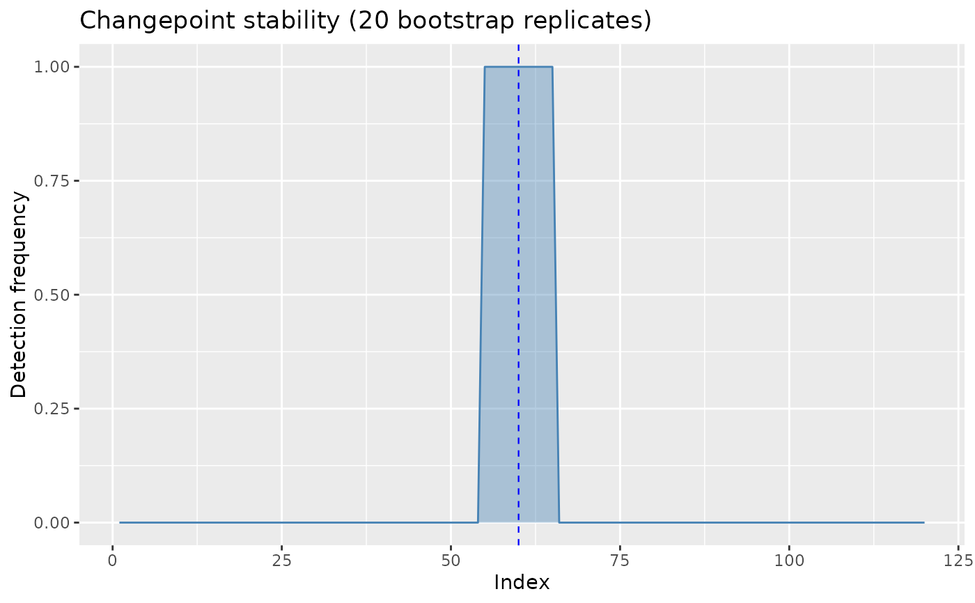
A ggcpt_stability object: a list with frequency (a tibble of index and freq, the proportion of replicates detecting a changepoint within margin of that index), original (the point-estimate ggcpt), and B. Methods: print() and autoplot() (frequency profile with the original detections marked).

Examples

set.seed(2026)
x <- c(rnorm(60), rnorm(60, 4))
st <- cpt_stability(x, method = "pelt", B = 20)
st
#> ggcpt_stability (20 bootstrap replicates, method: pelt)
#> 
#> Original changepoints and their re-detection frequency:
#> # A tibble: 1 × 2
#>      cp stability
#>   <int>     <dbl>
#> 1    60         1
ggplot2::autoplot(st)