
Wraps segmented::segmented() (Muggeo, 2003, 2008): maximum
likelihood estimation of continuous piecewise-linear
("broken-line") regressions, with standard errors and confidence
intervals for the breakpoint locations. Where the step-change engines
model jumps in the level, segmented models kinks in the trend, so
change_in is "slope" and the fitted broken line is stored in
the fitted column for autoplot(show_fit = TRUE).
Usage
segmented_wrapper(
  x,
  npsi = 1,
  conf_level = 0.95,
  seed = NULL,
  data = NULL,
  seg_z = NULL,
  family = c("gaussian", "poisson", "binomial"),
  ...
)
Arguments
- x
A numeric vector (a line in time is segmented), or a model formula (supply
data).- npsi
Number of breakpoints to estimate. Defaults to
1.- conf_level
Confidence level for breakpoint intervals. Defaults to
0.95.- seed
Optional seed (the estimator uses bootstrap restarting). The seed is scoped to this call:
.Random.seedis saved and restored, so a seeded call inside a simulation loop does not pin the loop's own stream.- data
A data frame, for formula input.
- seg_z
For formula input, the covariate whose relationship with the response breaks: its name, or a one-sided formula (
~ t) as segmented's ownseg.Ztakes it. Defaults to the formula's only numeric covariate, and must be named when there are several.- family
"gaussian"(a linear model, the default),"poisson"or"binomial"(a generalised linear model on the log or logit scale).- ...
Additional arguments passed to
segmented::segmented(), for examplepsi(starting values) orfixed.psi.
Value
A ggcpt object with ci_lower/ci_upper columns
and the fitted broken line in $data$fitted. Breakpoints are
rounded to the nearest index; for a continuous fit the reported location
is the kink itself. A constant series has no kink and returns an empty
result, rather than the arbitrary breakpoint a singular fit would give.
Formula input adds psi, psi_lower and psi_upper
(the breakpoints on the covariate's scale) and a $coefficients
table with the slope of seg_z in each segment.
Details
Called with a numeric vector it segments a line in time. Called with a
formula and data it does what the engine exists for: breakpoints
in the relationship between the response and a covariate,
seg_z. The result is then ordered by that covariate, which
becomes its index, so tidy()'s cp_index and the plot speak
in the covariate's units, and psi, psi_lower and
psi_upper give the breakpoints on that scale exactly.
References
Muggeo VM (2003). “Estimating regression models with unknown break-points.” Statistics in Medicine, 22(19), 3055–3071.
Muggeo VM (2008). “segmented: An R package to fit regression models with broken-line relationships.” R News, 8(1), 20–25.
See also
Other changepoint engines:
bcp_wrapper(),
beast_wrapper(),
bfast_wrapper(),
binsegrcpp_wrapper(),
bocpd_wrapper(),
cpm_wrapper(),
cpop_wrapper(),
cpt_wrapper(),
decafs_wrapper(),
ecp_wrapper(),
envcpt_wrapper(),
esac_wrapper(),
fabisearch_wrapper(),
fastcpd_wrapper(),
fcov_wrapper(),
fmean_wrapper(),
fpop_wrapper(),
geomcp_wrapper(),
hdcov_wrapper(),
hdreg_wrapper(),
idetect_wrapper(),
inspect_wrapper(),
kcp_wrapper(),
kwc_wrapper(),
mcp_wrapper(),
mosum_wrapper(),
network_wrapper(),
not_wrapper(),
npmojo_wrapper(),
nsp_wrapper(),
ocd_wrapper(),
pilliat_wrapper(),
smuce_wrapper(),
sn_wrapper(),
strucchange_wrapper(),
taylor_wrapper(),
tguh_wrapper(),
trend_wrapper(),
var_wrapper(),
wbs2_wrapper(),
wbs_wrapper(),
wbsts_wrapper()
Examples
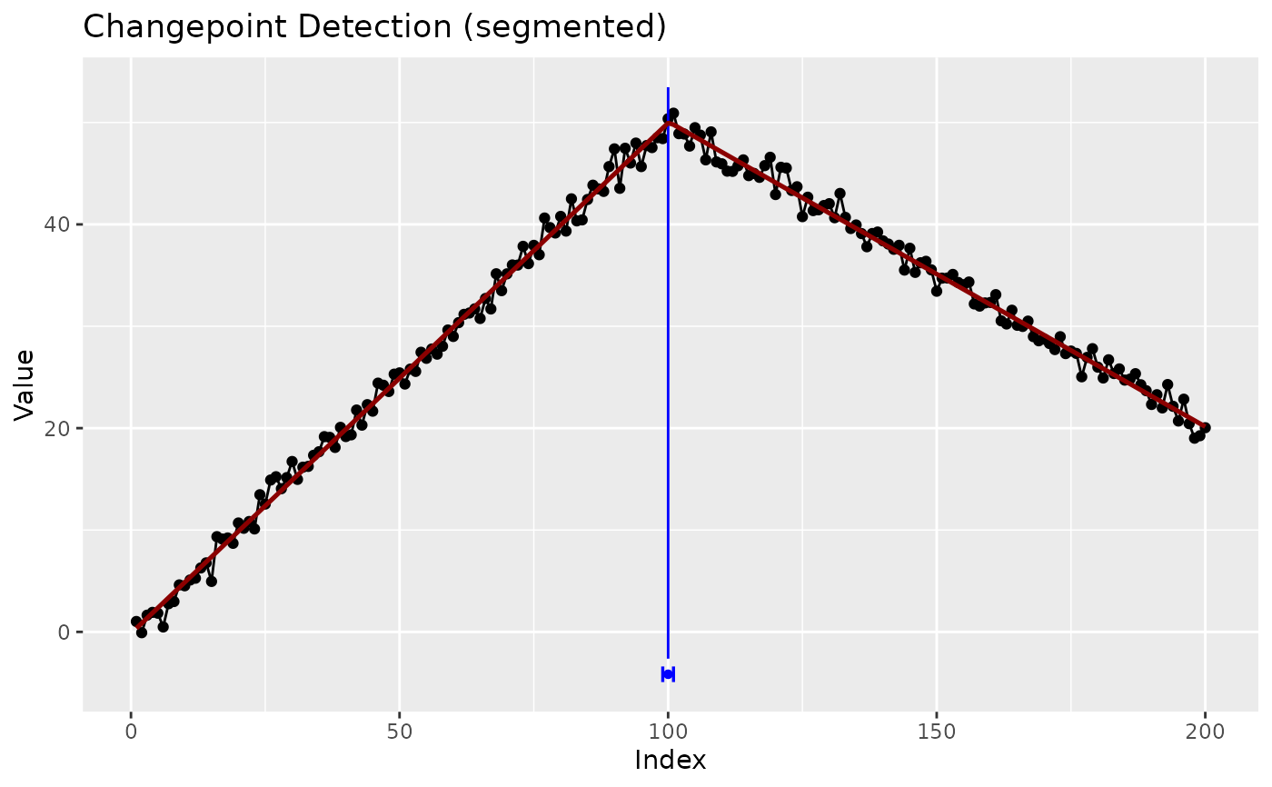
set.seed(2026)
y <- cumsum(c(rep(0.5, 100), rep(-0.3, 100))) + rnorm(200)
res <- segmented_wrapper(y, npsi = 1)
res$changepoints
#> # A tibble: 1 × 4
#> cp cp_value ci_lower ci_upper
#> <int> <dbl> <int> <int>
#> 1 100 50.4 99 101
ggplot2::autoplot(res, show_fit = TRUE, show_ci = TRUE)
 # A breakpoint in a dose-response relationship
d <- data.frame(dose = runif(150, 0, 10))
d$response <- 2 + 0.8 * pmin(d$dose, 6) + rnorm(150, 0, 0.4)
fit <- segmented_wrapper(response ~ dose, data = d)
fit$changepoints[, c("cp", "psi", "psi_lower", "psi_upper")]
#> # A tibble: 1 × 4
#> cp psi psi_lower psi_upper
#> <int> <dbl> <dbl> <dbl>
#> 1 94 6.01 5.69 6.33
# A breakpoint in a dose-response relationship
d <- data.frame(dose = runif(150, 0, 10))
d$response <- 2 + 0.8 * pmin(d$dose, 6) + rnorm(150, 0, 0.4)
fit <- segmented_wrapper(response ~ dose, data = d)
fit$changepoints[, c("cp", "psi", "psi_lower", "psi_upper")]
#> # A tibble: 1 × 4
#> cp psi psi_lower psi_upper
#> <int> <dbl> <dbl> <dbl>
#> 1 94 6.01 5.69 6.33