ggchangepoint: A Unified Tidy Interface for Changepoint Analysis in R

Youzhi Yu
University of Chicago

Abstract

ggchangepoint provides a unified, tidy interface to changepoint detection across the methodological spectrum. It introduces a single S3 result class, ggcpt, with broom-style methods (tidy(), glance(), augment()) (Robinson 2017), a central dispatcher cpt_detect() covering 31 detection methods across six algorithmic families, and native ggplot2 (Wickham 2016) visualisation through autoplot() and a set of composable geoms. Where a method quantifies its uncertainty — the simultaneous confidence intervals of SMUCE (Frick et al. 2014), the break-date intervals of Bai–Perron (Bai and Perron 1998), the posterior distributions of Bayesian detectors (Barry and Hartigan 1993; Adams and MacKay 2007) — the result object carries that uncertainty and the plotting layer can draw it. The package further supplies a penalty-path diagnostic (CROPS), batch detection over panels of series, bootstrap stability diagnostics, accuracy metrics aligned with current benchmarking conventions (van den Burg and Williams 2020), ground-truth simulation, and per-method citations. This article sets out the statistical background, the design of the package, and each method family in turn, with worked examples throughout.

Introduction

Changepoint analysis — locating the instants at which the stochastic behaviour of an ordered sequence changes — is one of the oldest problems in statistics, dating back at least to the continuous-inspection schemes of Page (1954), and one of its most active: recent surveys catalogue dozens of methods (Truong et al. 2020; Aminikhanghahi and Cook 2017). Its applications span virtually every domain that produces sequential data, including genomics (Picard et al. 2005), finance (Athey et al. 2022), climate science (Haslett and Raftery 1989), and signal processing (Lavielle 2005).

The R ecosystem mirrors this breadth. Penalised optimal partitioning lives in changepoint (Killick and Eckley 2014) and fpop (Maidstone et al. 2017); wild binary segmentation in wbs and breakfast (Fryzlewicz 2014, 2020); multiscale inference in stepR (Frick et al. 2014); Bayesian analysis in bcp (Erdman and Emerson 2007) and ocp (Adams and MacKay 2007); structural breaks in strucchange (Zeileis et al. 2002); and so on. Each of these packages is excellent at what it does, and each returns a different object, follows a different indexing convention, and draws (or does not draw) its own plots.

An analyst who wants to compare a PELT segmentation with a Bayesian posterior and a multiscale confidence set — a routine task in applied work — must therefore learn several APIs, reconcile several conventions, and write custom plotting code for each. ggchangepoint removes that friction. Its design goals are:

1. One vocabulary. A single front door, cpt_detect(x, method, change_in, penalty, ...), whose arguments mean the same thing for every engine.
2. One result type. Every detector returns a ggcpt object with a stable tidy contract, whatever the upstream engine returned.
3. One rendering path. Every result — point estimates, confidence intervals, fitted signals, posteriors, penalty paths — draws with autoplot() and extends with ordinary ggplot2 layers.
4. Wrap, don’t reinvent. All detection is delegated to the peer-reviewed upstream engines; optional engines live in Suggests and are loaded only when requested.

The changepoint problem

Let $y_{1:n} = (y_1, \dots, y_n)$ be an ordered sequence. A segmentation with $m$ changepoints is an ordered set $\tau_{1:m}$ satisfying $0 = \tau_0 < \tau_1 < \dots < \tau_m < \tau_{m+1} = n$, which partitions the data into the $m + 1$ segments $y_{(\tau_{i-1}+1):\tau_i}$, $i = 1, \dots, m+1$. Both the number of changepoints and their locations are unknown, and estimating them jointly is what makes the problem hard. Throughout the package a changepoint $\tau$ is reported as the last index of the left segment (the convention of the changepoint package), so the admissible locations are $1, \dots, n-1$; results from engines using the opposite convention are shifted on the way in, and the convention is recorded on every result object.

Penalised cost minimisation

The classical formulation chooses the segmentation minimising a penalised cost, $$\min_{m,\ \tau_{1:m}} \; \sum_{i=1}^{m+1} \mathcal{C}\!\left(y_{(\tau_{i-1}+1):\tau_i}\right) \;+\; \beta m,$$ where $\mathcal{C}$ is a segment cost — for a change in mean under Gaussian noise the residual sum of squares, more generally twice the negative maximised log-likelihood of the segment — and $\beta > 0$ is the price of each additional changepoint. Writing $k$ for the number of parameters a changepoint introduces, the familiar choices are $\beta = 2k$ (AIC) and $\beta = k \log n$ (BIC, or SIC in the changepoint literature) (Yao 1988), alongside the strengthened and modified variants discussed below. Solved naively by dynamic programming, the minimisation costs $O(n^2)$; PELT (Killick et al. 2012) prunes candidate changepoints to reach linear expected cost while remaining exact, and FPOP (Maidstone et al. 2017) reaches comparable speed by functional pruning.

Search-based and multiscale methods

A complementary family locates changepoints by scanning test statistics. Binary segmentation (Scott and Knott 1974; Vostrikova 1981) recursively splits the series at the maximal CUSUM statistic; wild binary segmentation (Fryzlewicz 2014) and its successor WBS2 (Fryzlewicz 2020) draw random subintervals so that short segments are not masked; narrowest-over-threshold (NOT) (Baranowski et al. 2019) favours the narrowest interval on which the contrast exceeds a threshold, which generalises cleanly to changes in slope; MOSUM (Eichinger and Kirch 2018) scans a moving-sum statistic at a fixed bandwidth, or across a range of bandwidths; Isolate–Detect (Anastasiou and Fryzlewicz 2022) isolates each changepoint in an expanding interval; and TGUH (Fryzlewicz 2022) performs a tail-greedy bottom-up merge. SMUCE (Frick et al. 2014) occupies a special place: it estimates the step function with the fewest jumps that still passes a simultaneous multiscale test at level $\alpha$, and in doing so delivers confidence intervals for every changepoint location — uncertainty statements most competitors cannot make. HSMUCE (Pein et al. 2017) extends this to heterogeneous noise.

Beyond the mean

Changes need not be in the mean: the change_in argument accepts "mean", "var", "meanvar", "slope", and "distribution". Nonparametric engines (energy statistics (Matteson and James 2014), nonparametric cost functions (Haynes et al. 2017), kernel running statistics (Arlot et al. 2019; Cabrieto et al. 2018), joint characteristic functions (McGonigle and Cho 2025), self-normalisation (Zhao et al. 2022)) detect distributional change without likelihood assumptions; Bayesian engines (Barry and Hartigan 1993; Adams and MacKay 2007; Zhao et al. 2019) return posteriors instead of point sets; high-dimensional engines (Wang and Samworth 2018; Chen et al. 2022; Grundy et al. 2020) aggregate evidence across coordinates; and regression engines (Bai and Perron 1998; Muggeo 2003) date breaks in model coefficients. The tour below visits each family with runnable code.

Design of the package

The ggcpt result contract

Every detector returns an object of class ggcpt containing:

• changepoints: a tibble with one row per changepoint. Columns cp (location, “left” convention) and cp_value (the data value at cp) are always present; engines add ci_lower/ci_upper (SMUCE, HSMUCE, strucchange, segmented), posterior_prob (bcp, BEAST), detection_time (CPM), strength (inspect), declared_at (ocd), or mapping (geomcp) when they have more to say.
• segments: a tibble of the induced segments (seg_id, start, end, n, param_estimate).
• data: the analysed series as a tibble (index, value), plus a fitted column when the engine estimates a signal (SMUCE, DeCAFS, CPOP, segmented, bcp, BEAST).
• method, change_in, penalty (a list(type, value) descriptor), cp_convention (always "left"), runtime (elapsed seconds, timed by cpt_detect() and NA when a wrapper is called directly), and fit (the untouched upstream object, for experts).

Multivariate results additionally carry a data_wide tibble with one column per coordinate, which autoplot() renders as faceted small-multiples.

Tidy methods and the plotting layer

The class implements the full complement of generics R users expect:

set.seed(2022)
x <- c(rnorm(100, 0, 1), rnorm(100, 10, 1))
res <- cpt_detect(x, method = "pelt", change_in = "mean")
res
#> ggcpt (changepoint detection result)
#>   Method:          pelt 
#>   Change in:       mean 
#>   Changepoints found: 1 
#>   CP convention:   left 
#>   Penalty:         MBIC 
#>   Series length:   200 
#> 
#> Changepoints:
#> # A tibble: 1 × 2
#>      cp cp_value
#>   <int>    <dbl>
#> 1   100    0.467
tidy(res)
#> # A tibble: 1 × 2
#>      cp cp_value
#>   <int>    <dbl>
#> 1   100    0.467
glance(res)
#> # A tibble: 1 × 9
#>       n n_changepoints method change_in penalty_type penalty_value cp_convention
#>   <int>          <int> <chr>  <chr>     <chr>                <dbl> <chr>        
#> 1   200              1 pelt   mean      MBIC                    NA left         
#> # ℹ 2 more variables: total_cost <dbl>, runtime <dbl>
head(augment(res))
#> # A tibble: 6 × 6
#>   index  value seg_id .fitted .resid is_changepoint
#>   <int>  <dbl>  <int>   <dbl>  <dbl> <lgl>         
#> 1     1  0.900      1   0.139  0.761 FALSE         
#> 2     2 -1.17       1   0.139 -1.31  FALSE         
#> 3     3 -0.897      1   0.139 -1.04  FALSE         
#> 4     4 -1.44       1   0.139 -1.58  FALSE         
#> 5     5 -0.331      1   0.139 -0.470 FALSE         
#> 6     6 -2.90       1   0.139 -3.04  FALSE

autoplot() draws the series, the changepoint rules, and — on request — the fitted segment means (show_segments), the engine’s fitted signal (show_fit), and changepoint-location confidence intervals (show_ci):

autoplot(res, show_segments = TRUE)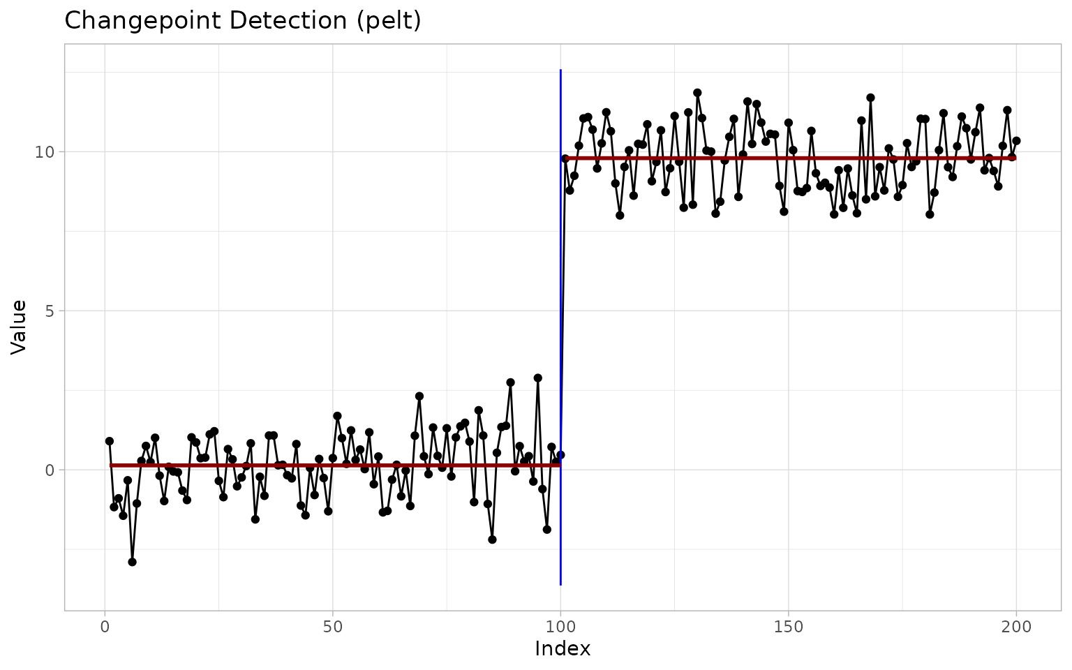

Composable layers (geom_changepoint(), geom_cpt_segment(), geom_cpt_ci(), stat_changepoint()), a theme (theme_ggcpt()), and segment shading (annotate_segments()) let the same results be built into bespoke graphics; summary(), as_tibble(), as.data.frame(), format(), and plot() complete the S3 surface.

Design principles

The four goals above are recorded in the package as principles P1 — wrap, don’t reinvent (bind to peer-reviewed CRAN engines), P2 — tidy in, tidy out (stable column names across all methods), P3 — ggplot2 all the way down (every result renders and extends), and P4 — one vocabulary (x, method, change_in, penalty, ...). Three further principles govern how the interface evolves:

• P5 — Progressive disclosure: beginners call cpt_detect() + autoplot(); experts reach the upstream fit via $fit.
• P6 — No surprises: the 0.1.0 functions still work unchanged.
• P7 — Document everything you ship: every export is introduced in the README and a vignette.

Release 0.4.0 adds an eighth: P8 — carry the uncertainty. Where a method quantifies uncertainty, the ggcpt object records it and autoplot() can draw it.

The unified dispatcher

cpt_detect() dispatches by method name; cpt_methods() reports every method the package knows, its engine, what it can detect, and whether the engine is installed:

cpt_methods()
#> # A tibble: 35 × 6
#>    method   change_in                   engine   status target_release installed
#>    <chr>    <chr>                       <chr>    <chr>  <chr>          <lgl>    
#>  1 pelt     mean, var, meanvar          changep… avail… NA             TRUE     
#>  2 binseg   mean, var, meanvar          changep… avail… NA             TRUE     
#>  3 segneigh mean, var, meanvar          changep… avail… NA             TRUE     
#>  4 amoc     mean, var, meanvar          changep… avail… NA             TRUE     
#>  5 np       distribution                changep… avail… NA             TRUE     
#>  6 ecp      distribution (multivariate) ecp      avail… NA             TRUE     
#>  7 fpop     mean                        fpop     avail… NA             TRUE     
#>  8 wbs      mean                        wbs      avail… NA             TRUE     
#>  9 wbs2     mean                        breakfa… avail… NA             TRUE     
#> 10 not      mean, var, slope            not      avail… NA             TRUE     
#> # ℹ 25 more rows

Requests are validated against this capability matrix: asking a mean-only engine for a variance change is an error with the legal alternatives named — never a silent substitution. Univariate methods likewise refuse multi-column input rather than flattening it.

Penalty semantics differ across engines, and cpt_penalty() documents and constructs the standard values:

cpt_penalty("BIC", n = 200)
#> [1] 5.298317
cpt_penalty("MBIC", n = 200)
#> [1] 10.59663
cpt_penalty("Hannan-Quinn", n = 200)
#> [1] 3.334779
cpt_penalty("sSIC", n = 200)
#> [1] 5.387402

Two of these warrant a word. "sSIC" is the strengthened Schwarz criterion $k (\log n)^{\alpha}$, with $\alpha = 1.01$ by default (Fryzlewicz 2014) — marginally heavier than BIC, and the criterion the search-based engines apply internally. "MBIC" in cpt_penalty() returns $0.5 (k+1) \log n + \log \binom{n}{k}$: a BIC-type term plus the combinatorial cost of placing $k$ changepoints among $n$ observations. It is deliberately stronger than "BIC", but it is not the modified BIC of Zhang and Siegmund (2007), whose penalty $1.5 k \log n + 0.5 \sum_i \log(\ell_i / n)$ depends on the segment lengths $\ell_i$ and therefore cannot be written as a function of $n$ and $k$ alone; nor is it the quantity the changepoint package computes for its own character penalty "MBIC".

Character penalties ("MBIC", "BIC", …) pass through to the changepoint-family engines natively and are resolved to numeric values for the functional-pruning engines (fpop, cpop, decafs). Search-based engines (WBS, NOT, MOSUM, …) select their own models and ignore the argument, as do the engines tuned by a significance level, a posterior-probability threshold, or an average run length (SMUCE, bcp, BEAST, CPM, SNSeg).

A tour of the method families

Throughout we use simulated series with known truth, so that results can be checked by eye. cpt_simulate() draws series with prescribed changepoints, and five canonical test signals ship as ready-made generators: signal_blocks() (the Donoho–Johnstone blocks signal (Donoho and Johnstone 1994)), signal_fms(), signal_teeth(), signal_stairs(), and signal_mix(). The comparison vignette puts them to work. The sections that follow work through six families — penalised and optimal partitioning, multiscale and search, Bayesian, nonparametric and sequential, multivariate and high-dimensional, and regression-based — plus two concerns that cut across all of them: change in slope, and robustness to drift, autocorrelation and model ambiguity.

set.seed(2026)
x_mean  <- c(rnorm(100), rnorm(100, 4))                # mean shift at 100
x_multi <- c(rnorm(100), rnorm(100, 3), rnorm(100, -1)) # shifts at 100, 200
x_slope <- cumsum(c(rep(0.4, 100), rep(-0.3, 100))) + rnorm(200) # kink at 100

Penalised and optimal partitioning

PELT (Killick et al. 2012), binary segmentation (Scott and Knott 1974), segment neighbourhoods (Auger and Lawrence, 1989), and at-most-one-change (AMOC; Hinkley, 1970) come from the changepoint package (Killick and Eckley 2014); FPOP (Maidstone et al. 2017) from fpop:

tidy(cpt_detect(x_multi, method = "pelt"))
#> # A tibble: 2 × 2
#>      cp cp_value
#>   <int>    <dbl>
#> 1   100   -0.100
#> 2   200    1.90
tidy(cpt_detect(x_multi, method = "binseg"))
#> # A tibble: 2 × 2
#>      cp cp_value
#>   <int>    <dbl>
#> 1   100   -0.100
#> 2   201    0.337

tidy(cpt_detect(x_multi, method = "fpop"))
#> # A tibble: 2 × 2
#>      cp cp_value
#>   <int>    <dbl>
#> 1   100   -0.100
#> 2   200    1.90

The Achilles heel of penalised methods is the choice of $\beta$. Rather than committing to one value, cpt_crops() computes every optimal segmentation as $\beta$ ranges over an interval — the CROPS algorithm of Haynes, Eckley and Fearnhead (2017), as implemented by changepoint — and turns penalty selection into a diagnostic:

path <- cpt_crops(x_multi)
path
#> ggcpt_path (CROPS penalty path)
#>   Change in:       mean 
#>   Penalty range:  [5.704, 57.04]
#>   Series length:   300 
#>   Distinct segmentations: 5 
#> 
#> # A tibble: 5 × 3
#>   penalty n_cpts  cost
#>     <dbl>  <int> <dbl>
#> 1    6.69      2  327.
#> 2    6.27      5  307.
#> 3    6.19      8  288.
#> 4    5.76      9  282.
#> 5    5.70     10  276.
autoplot(path)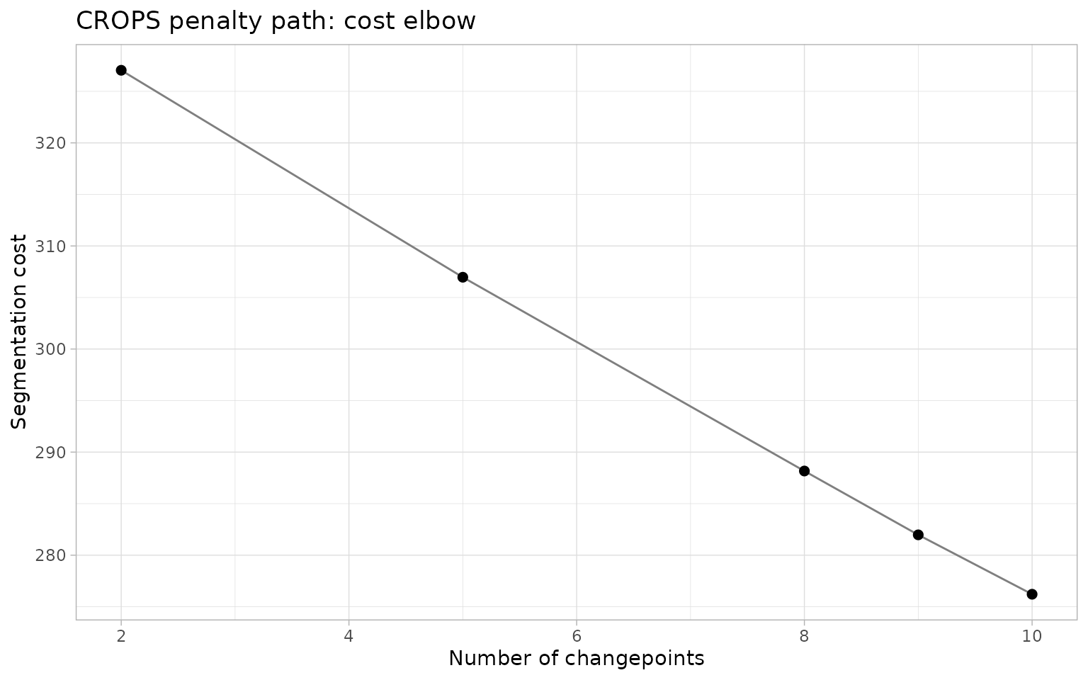

The default plot puts segmentation cost against model size, and the usual reading takes the model beyond which the cost stops falling appreciably. The sweep over the default interval $[\log n,\, 10 \log n]$ admits only a handful of distinct segmentations here, and the most parsimonious of them already recovers the two true changepoints. autoplot(path, type = "segmentations") shows the candidate models themselves, and autoplot(path, type = "path") the map from penalty to model size:

autoplot(path, type = "segmentations")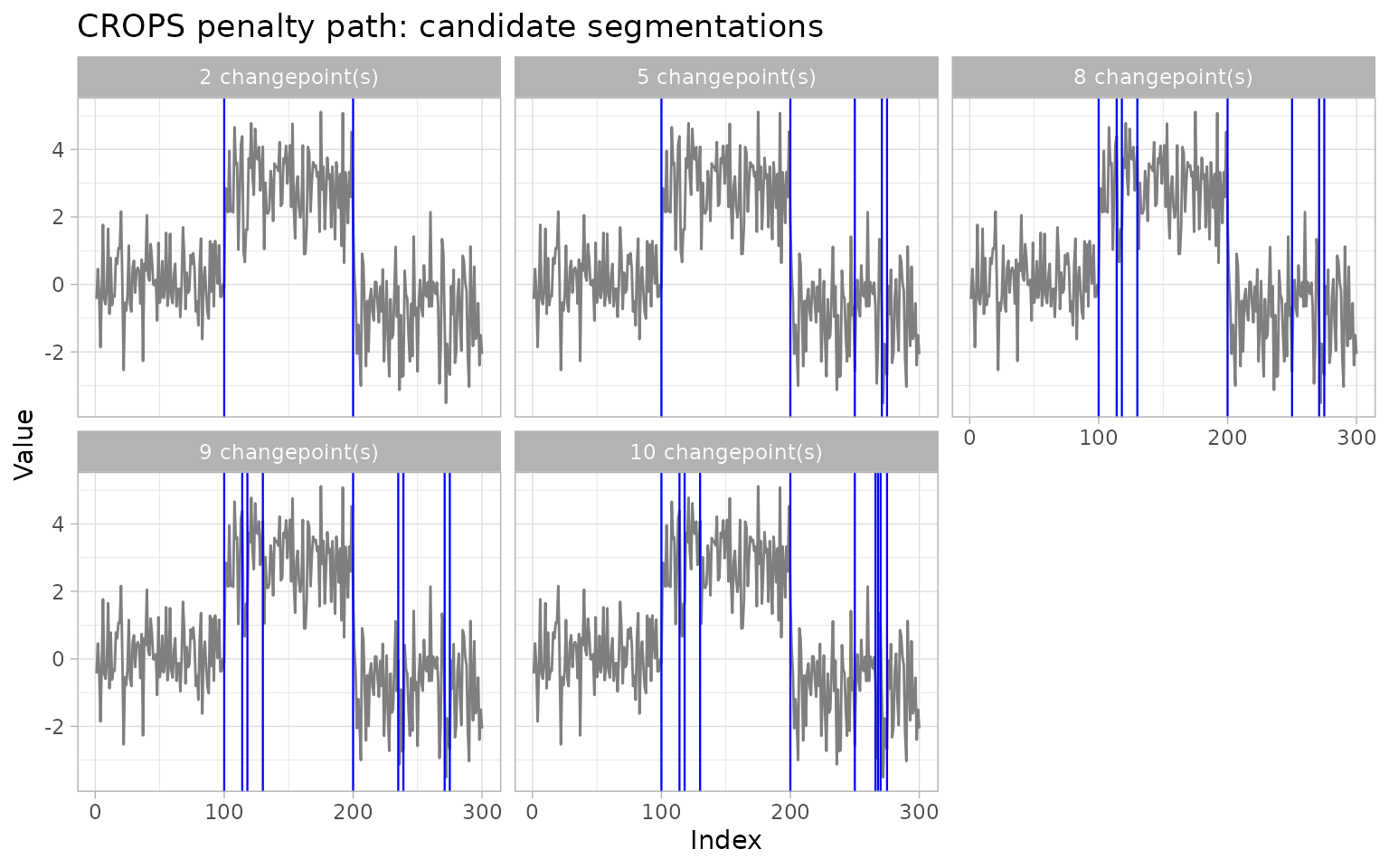

The modern fastcpd engine (Li and Zhang 2024) brings the same penalised formulation to a wide family of models — mean, variance, mean-and-variance, and AR/ARMA/GARCH model changes — with sequential-gradient-descent speed:

tidy(fastcpd_wrapper(x_multi, family = "mean"))
#> # A tibble: 2 × 2
#>      cp cp_value
#>   <int>    <dbl>
#> 1   100   -0.100
#> 2   200    1.90

Multiscale and search methods

The randomised and multiscale searchers are one call each, whether through cpt_detect() or through the wrapper directly:

tidy(wbs_wrapper(x_multi, seed = 1))
#> # A tibble: 2 × 2
#>      cp cp_value
#>   <int>    <dbl>
#> 1   100   -0.100
#> 2   200    1.90

tidy(not_wrapper(x_multi, seed = 1))
#> # A tibble: 2 × 2
#>      cp cp_value
#>   <int>    <dbl>
#> 1   100   -0.100
#> 2   200    1.90

tidy(mosum_wrapper(x_multi))
#> # A tibble: 2 × 2
#>      cp cp_value
#>   <int>    <dbl>
#> 1   100   -0.100
#> 2   200    1.90

tidy(idetect_wrapper(x_multi, seed = 1))
#> # A tibble: 2 × 2
#>      cp cp_value
#>   <int>    <dbl>
#> 1   100   -0.100
#> 2   200    1.90
tidy(wbs2_wrapper(x_multi))
#> # A tibble: 2 × 2
#>      cp cp_value
#>   <int>    <dbl>
#> 1   100   -0.100
#> 2   200    1.90
tidy(tguh_wrapper(x_multi))
#> # A tibble: 2 × 2
#>      cp cp_value
#>   <int>    <dbl>
#> 1   100   -0.100
#> 2   199    4.53

SMUCE (Frick et al. 2014) is the family’s inferential flagship: its level $\alpha$ bounds the probability of overestimating the number of changepoints (the default is alpha = 0.5, stepR’s own recommendation for estimation rather than testing), and every location comes with a confidence interval, stored in ci_lower/ci_upper and drawn by show_ci = TRUE as whiskers near the foot of the panel (the step fit is drawn by show_fit = TRUE):

res_smuce <- smuce_wrapper(x_multi)
tidy(res_smuce)
#> # A tibble: 2 × 4
#>      cp cp_value ci_lower ci_upper
#>   <int>    <dbl>    <int>    <int>
#> 1   100   -0.100       98      103
#> 2   200    1.90       199      202
autoplot(res_smuce, show_ci = TRUE, show_fit = TRUE)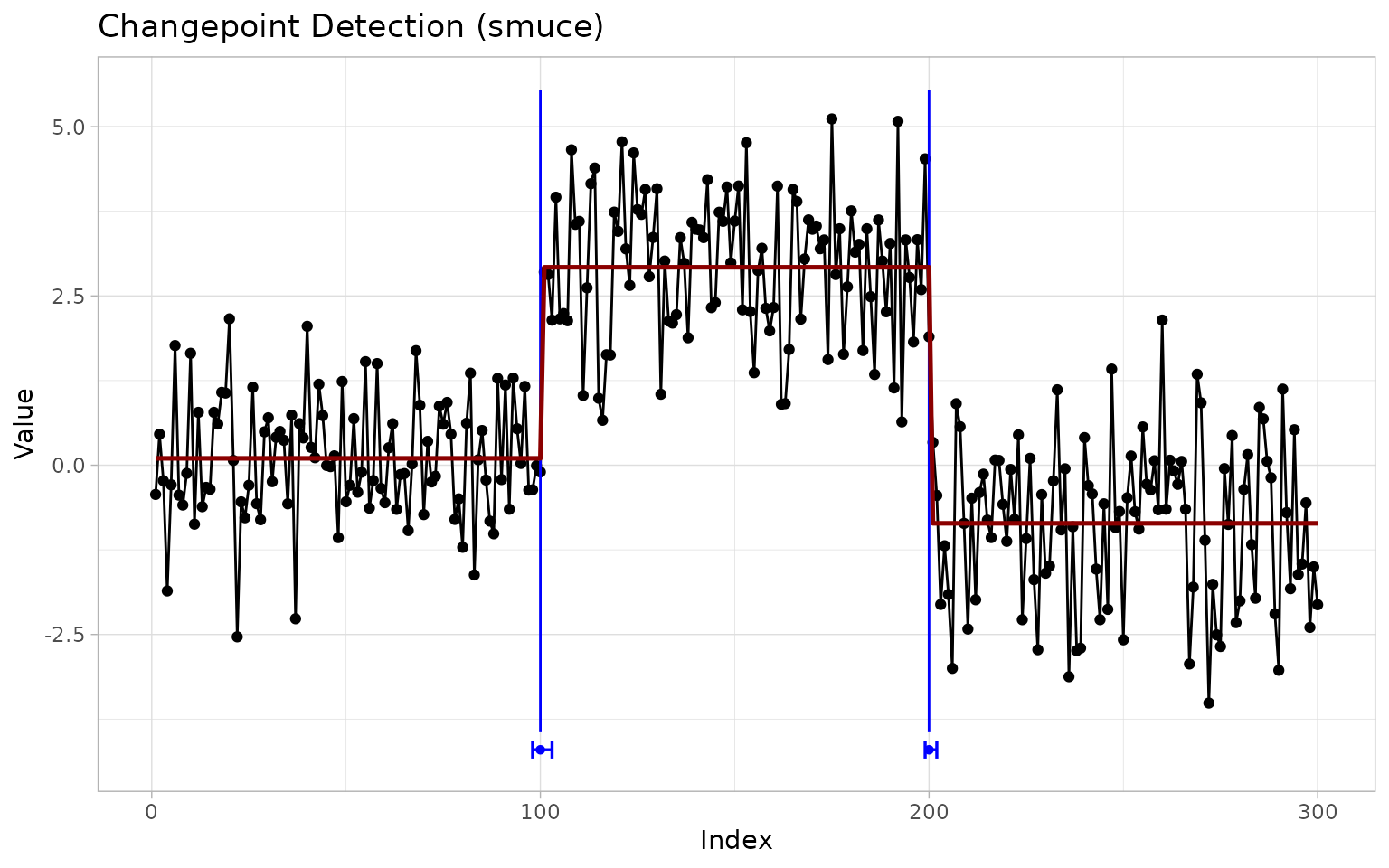

For heterogeneous noise, smuce_wrapper(x, family = "hsmuce") (or cpt_detect(x, method = "hsmuce")) runs HSMUCE (Pein et al. 2017).

Changes in slope

A kink in the trend is not a jump in the level, and running a mean-change detector on a trending series over-detects notoriously. CPOP (Fearnhead et al. 2019; Fearnhead and Grose 2024) solves the change-in-slope problem exactly under an $L_0$ penalty, returning a continuous piecewise-linear fit:

res_cpop <- cpop_wrapper(x_slope)
tidy(res_cpop)
#> # A tibble: 1 × 2
#>      cp cp_value
#>   <int>    <dbl>
#> 1   100     38.6
autoplot(res_cpop, show_fit = TRUE)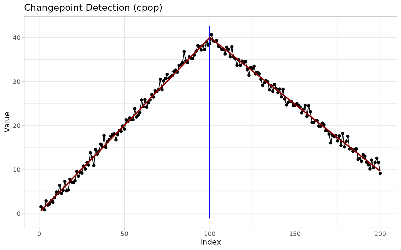

NOT with its linear contrast (Baranowski et al. 2019) offers a search-based alternative; the dispatcher routes cpt_detect(x, method = "not", change_in = "slope") to it automatically:

tidy(cpt_detect(x_slope, method = "not", change_in = "slope"))
#> # A tibble: 2 × 2
#>      cp cp_value
#>   <int>    <dbl>
#> 1    85     36.8
#> 2   101     40.7

Bayesian detection

The Barry–Hartigan product partition model (Barry and Hartigan 1993), via the bcp package (Erdman and Emerson 2007), returns a posterior probability of a changepoint at every location along with posterior segment means. Locations clearing prob_threshold populate the changepoints tibble (with their probabilities), and ggcpt_posterior() draws the classic two-panel display:

res_bcp <- bcp_wrapper(x_mean, seed = 2026)
tidy(res_bcp)
#> # A tibble: 1 × 3
#>      cp cp_value posterior_prob
#>   <int>    <dbl>          <dbl>
#> 1   100    0.369              1
ggcpt_posterior(res_bcp)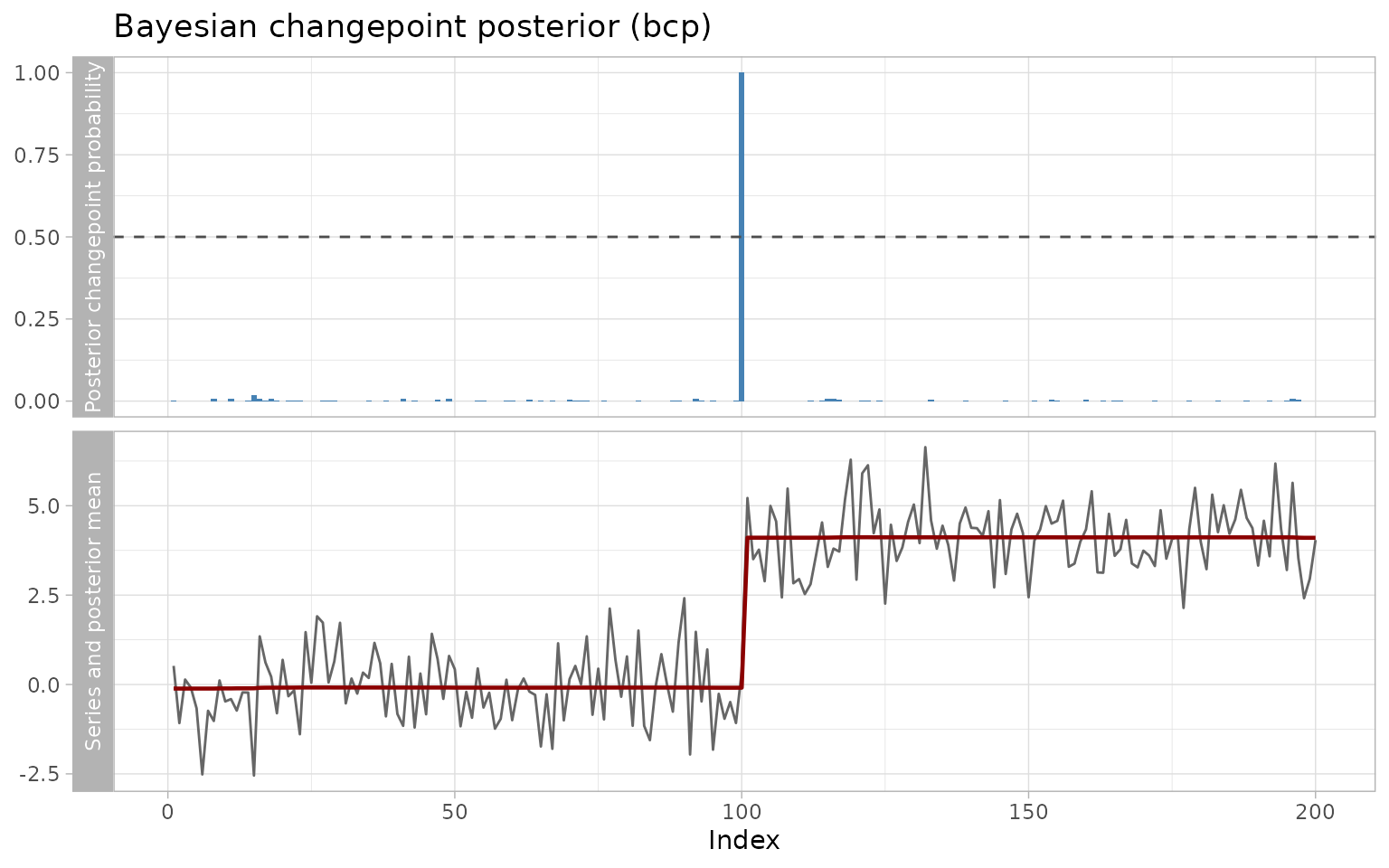

Bayesian online changepoint detection (Adams and MacKay 2007) instead tracks the posterior over the current run length — the time elapsed since the last change — updating it recursively as each observation arrives. Its signature graphic is the run-length heatmap, in which a change shows up as the posterior mass falling back to a run length of zero:

res_bocpd <- bocpd_wrapper(x_mean)
tidy(res_bocpd)
#> # A tibble: 1 × 2
#>      cp cp_value
#>   <int>    <dbl>
#> 1   100    0.369
ggcpt_runlength(res_bocpd)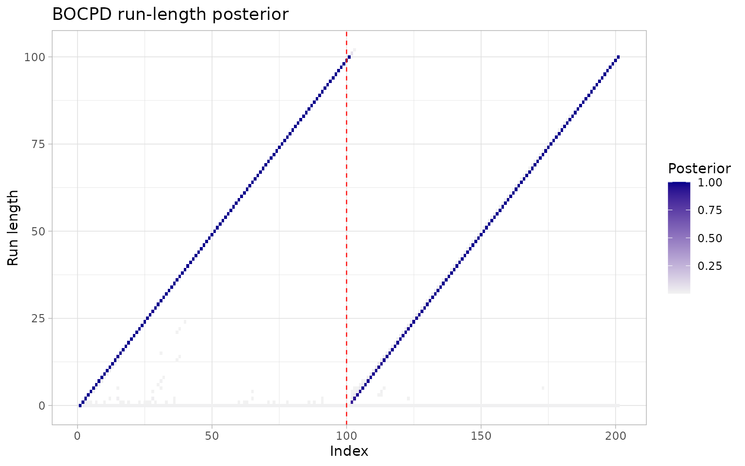

A third Bayesian engine, BEAST (Zhao et al. 2019) via Rbeast, averages over models rather than conditioning on one, and is wired as cpt_detect(x, method = "beast") (or beast_wrapper()); it too reports posterior_prob and renders with ggcpt_posterior().

Nonparametric and sequential detection

When no parametric form is trustworthy, the nonparametric cost approach of changepoint.np (Haynes et al. 2017) and the energy-statistics E-Divisive of ecp (Matteson and James 2014; James and Matteson 2014) detect general distributional change:

set.seed(2022)
tidy(cpt_detect(x_mean, method = "np"))
#> # A tibble: 1 × 2
#>      cp cp_value
#>   <int>    <dbl>
#> 1   100    0.369
tidy(cpt_detect(x_mean, method = "ecp", seed = 1))
#> # A tibble: 1 × 2
#>      cp cp_value
#>   <int>    <dbl>
#> 1   100    0.369

The cpm package (Ross 2015) recasts detection as a stream of two-sample tests (Mann–Whitney for location, Mood for scale, Lepage, Kolmogorov–Smirnov, Cramér–von Mises, and parametric variants), run here over the whole series in one pass to mimic an online monitor. Its results distinguish where a change happened (cp) from when it was detected (detection_time), the lag inherent in sequential monitoring:

tidy(cpm_wrapper(x_mean, cpm_type = "Mann-Whitney"))
#> # A tibble: 3 × 3
#>      cp cp_value detection_time
#>   <int>    <dbl>          <int>
#> 1    23   -1.39              30
#> 2    50    0.426             67
#> 3   100    0.369            104

Three further nonparametric engines are wired and worth knowing: kernel change-point analysis on running statistics (kcp_wrapper(), engine kcpRS), which detects changes in running means, variances, autocorrelations, or correlations (Arlot et al. 2019; Cabrieto et al. 2018); NP-MOJO (npmojo_wrapper(), engine CptNonPar), which detects changes in the marginal or lagged joint distribution while remaining valid under serial dependence (McGonigle and Cho 2025); and self-normalised segmentation (sn_wrapper(), engine SNSeg), which avoids long-run variance estimation altogether and tests changes in means, variances, autocorrelations, or bivariate correlations (Zhao et al. 2022).

Robustness to drift, autocorrelation, and model ambiguity

The most common failure of mean-change detection in practice is not a subtle statistical one: it is running a Gaussian-mean detector on data whose baseline drifts or whose noise is autocorrelated, and then reporting a changepoint wherever the model is wrong. DeCAFS (Romano et al. 2022) models exactly this regime — abrupt changes superimposed on random-walk drift and AR(1) noise — and separates the two:

res_decafs <- decafs_wrapper(x_mean)
tidy(res_decafs)
#> # A tibble: 1 × 2
#>      cp cp_value
#>   <int>    <dbl>
#> 1   100    0.369
autoplot(res_decafs, show_fit = TRUE)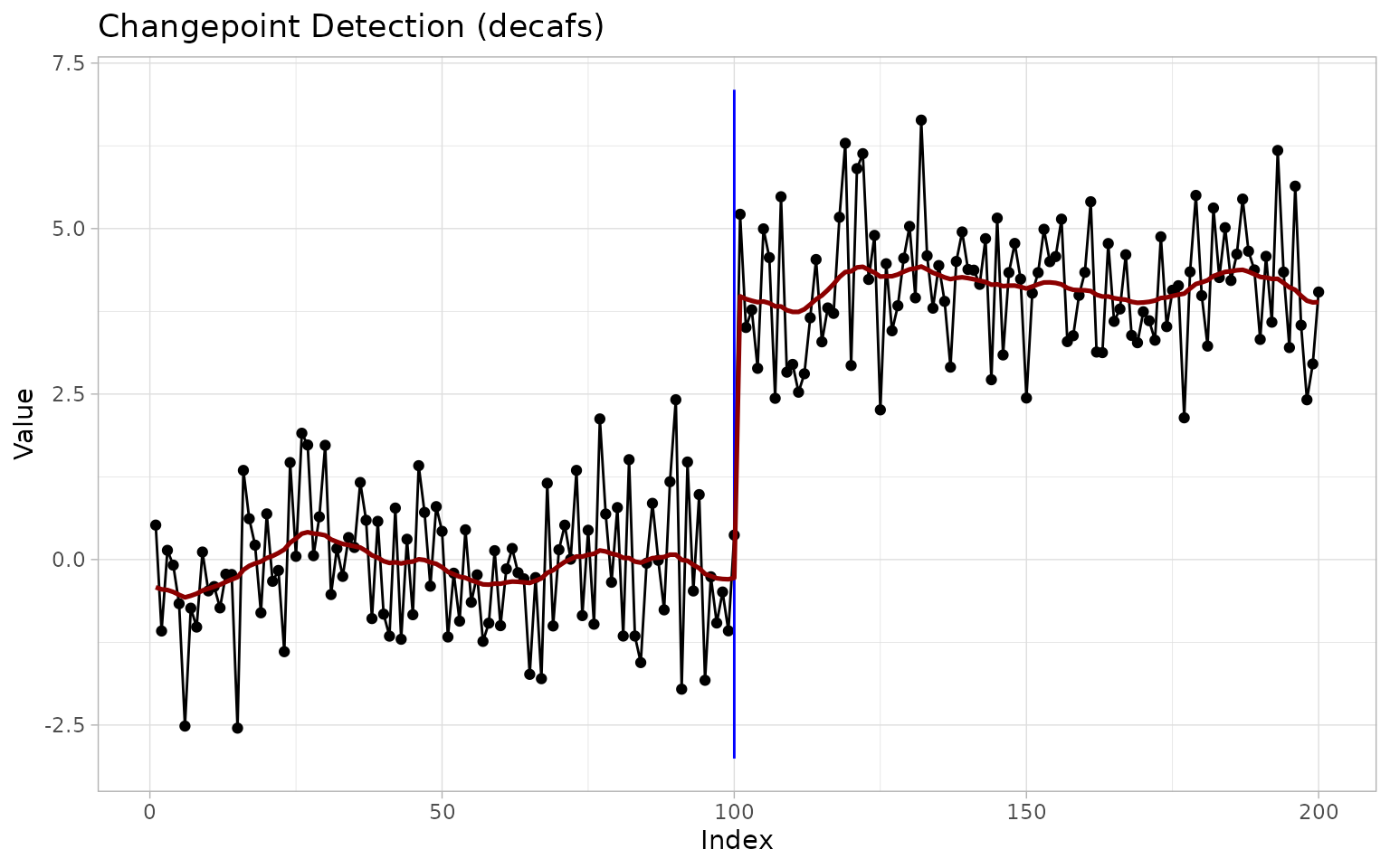

EnvCpt (Beaulieu and Killick 2018) attacks the same confusion by model selection: it fits up to twelve competing descriptions — constant mean or linear trend, each with or without changepoints, and with white-noise, AR(1) or AR(2) errors — and reports changepoints only if a changepoint model wins on an information criterion:

res_env <- envcpt_wrapper(x_mean, models = c("mean", "meancpt", "trendcpt"))
glance(res_env)
#> # A tibble: 1 × 9
#>       n n_changepoints method change_in penalty_type penalty_value cp_convention
#>   <int>          <int> <chr>  <chr>     <chr>                <dbl> <chr>        
#> 1   200              1 envcpt mean      AIC: meancpt          568. left         
#> # ℹ 2 more variables: total_cost <dbl>, runtime <dbl>

The winning model’s name is recorded in the penalty descriptor (penalty_type above, here AIC: meancpt), so “no changepoints, it’s just autocorrelation” is a first-class answer.

Multivariate and high-dimensional detection

Multivariate methods accept a matrix (rows are time points) directly. The energy-statistics E-Divisive of ecp was built for this (Matteson and James 2014); for high-dimensional data whose change is confined to a sparse subset of coordinates, inspect (Wang and Samworth 2018) finds an optimal sparse projection of the CUSUM matrix and reports the projected evidence (strength). Multivariate results render as faceted small-multiples with shared changepoint rules:

set.seed(2026)
X <- cbind(a = c(rnorm(80), rnorm(80, 3)),
           b = c(rnorm(80), rnorm(80, -2)),
           c = rnorm(160))
res_hd <- inspect_wrapper(X)
tidy(res_hd)
#> # A tibble: 1 × 3
#>      cp cp_value strength
#>   <int>    <dbl>    <dbl>
#> 1    80    0.785     21.9
autoplot(res_hd)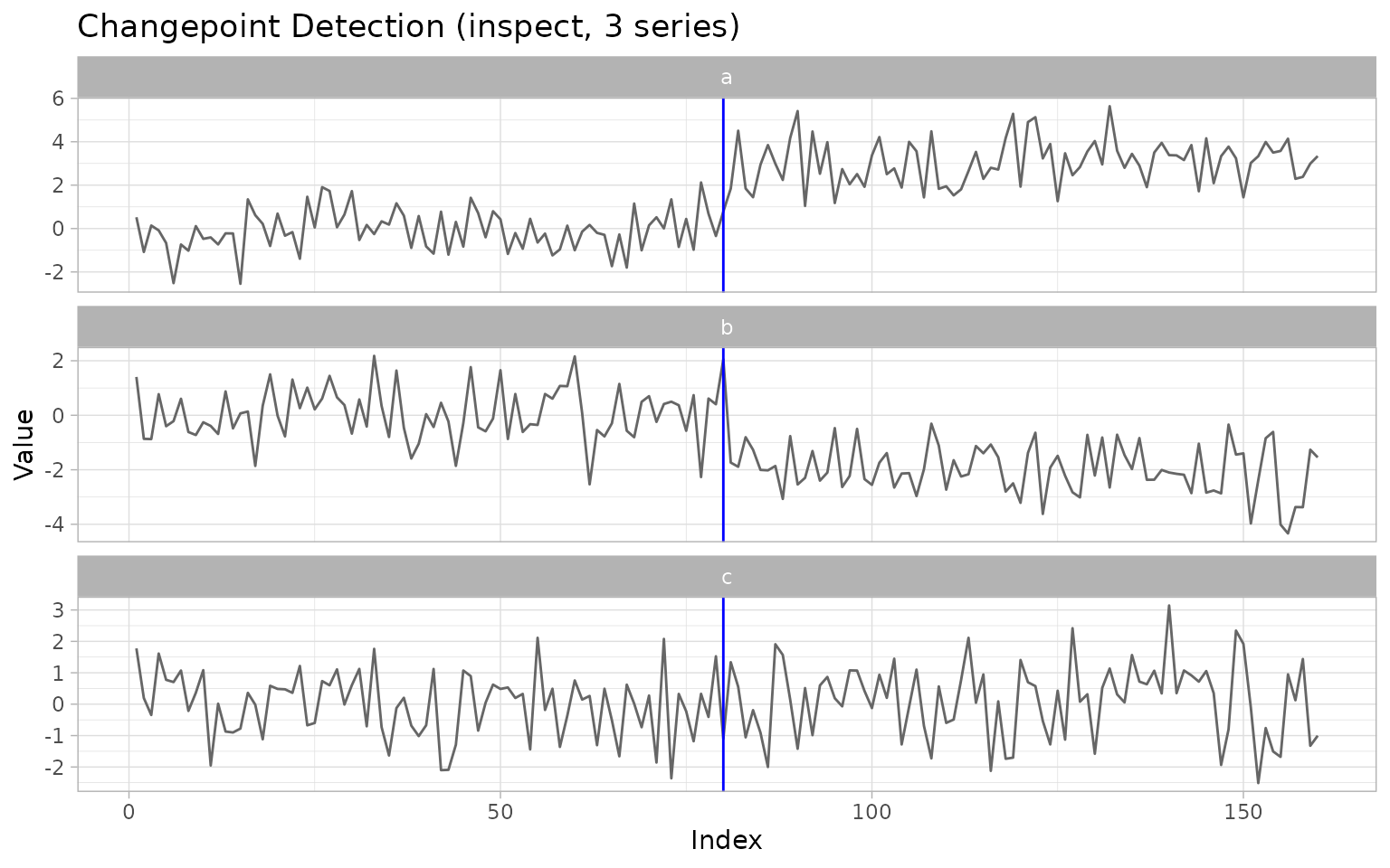

Two further engines complete the family. geomcp_wrapper() (engine changepoint.geo) maps each observation to its distance from and its angle to a reference point, then segments the two mapped series, catching changes in magnitude and in orientation respectively (Grundy et al. 2020). And ocd_wrapper() (engine ocd) monitors a high-dimensional stream online with worst-case detection-delay guarantees (Chen et al. 2022). Because detection there is sequential, the locations it reports are declaration times — the change plus the detection delay — recorded in declared_at; the wrapper estimates the pre-change baseline from an initial training window and resets after each declaration so that several changes can be found. Like the method itself, it needs at least two coordinates and refuses a single series.

Structural breaks in regression

Econometric practice dates breaks in regression coefficients. The Bai–Perron estimator (Bai and Perron 1998, 2003), via strucchange (Zeileis et al. 2002), returns break dates with confidence intervals; called on a bare series it dates mean shifts, and called with a formula it dates breaks in arbitrary regressions:

res_bp <- strucchange_wrapper(x_mean)
tidy(res_bp)
#> # A tibble: 1 × 4
#>      cp cp_value ci_lower ci_upper
#>   <int>    <dbl>    <int>    <int>
#> 1   100    0.369       99      101
autoplot(res_bp, show_ci = TRUE)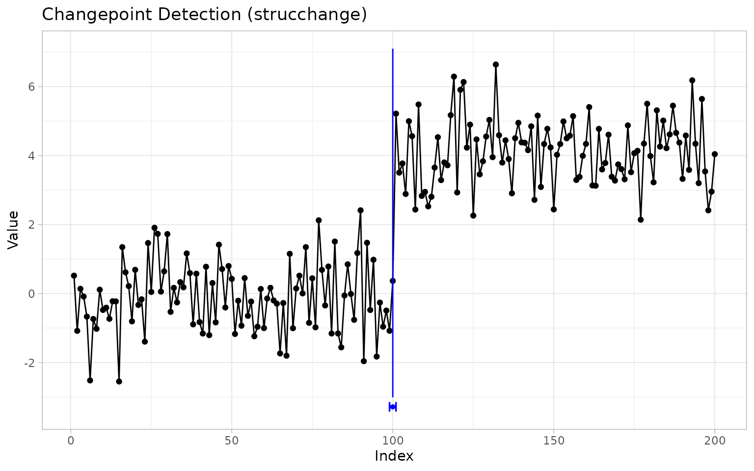

Where the regression function is continuous — a kink rather than a jump — segmented (Muggeo 2003, 2008) estimates broken-line relationships with standard errors for the breakpoints:

res_seg <- segmented_wrapper(x_slope, npsi = 1, seed = 1)
tidy(res_seg)
#> # A tibble: 1 × 4
#>      cp cp_value ci_lower ci_upper
#>   <int>    <dbl>    <int>    <int>
#> 1   100     38.6       98      101
autoplot(res_seg, show_fit = TRUE, show_ci = TRUE)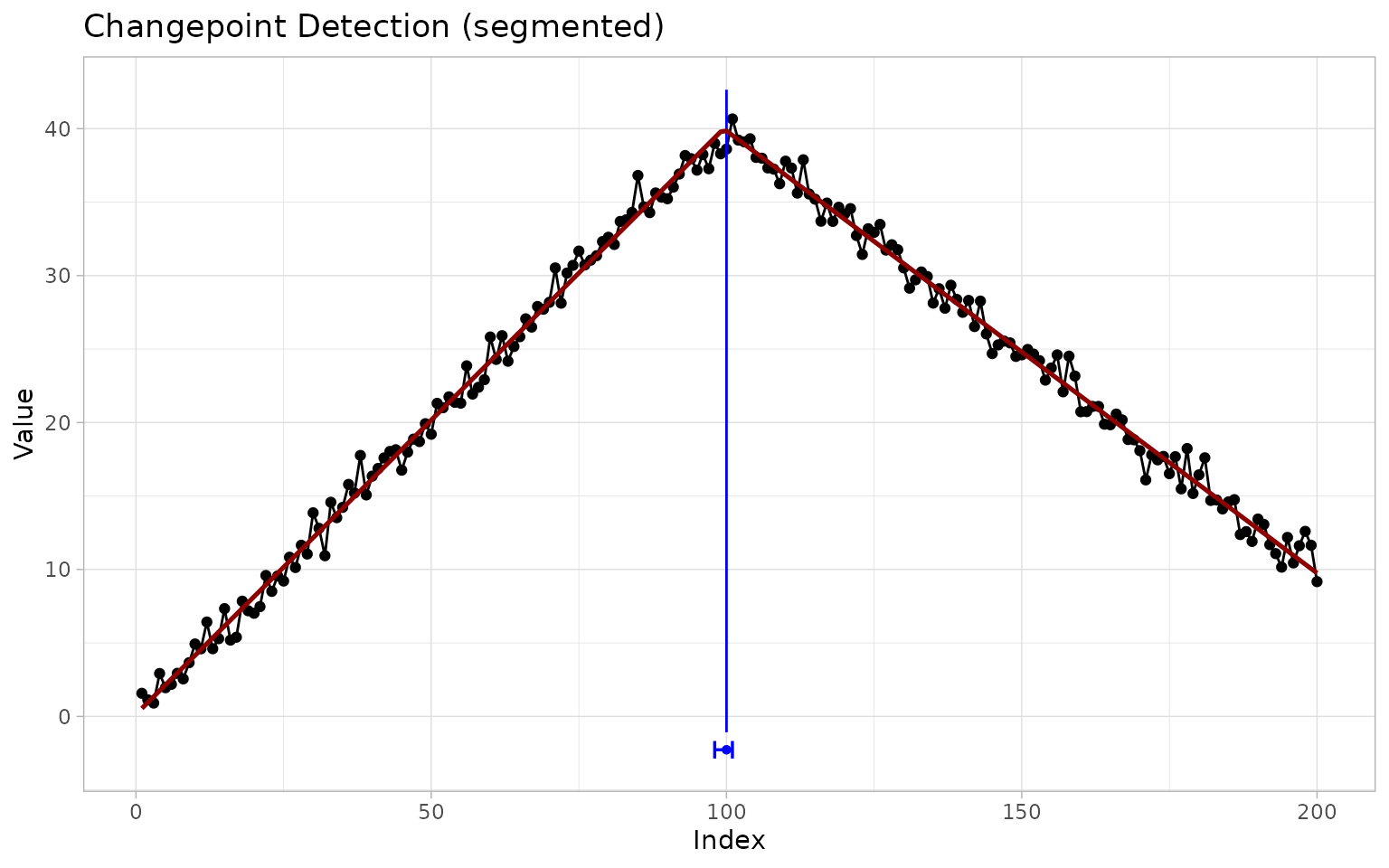

Beyond detection

Batch detection over many series

Applied work rarely stops at one series. cpt_batch() runs one detector over every column of a matrix or data frame (or every element of a list) and returns a tibble with one row per series, carrying both the tidy changepoints and the full ggcpt object in list-columns. With future and future.apply installed it honours a non-sequential future::plan(), using parallel-safe RNG:

set.seed(2026)
panel <- cbind(shifted = x_mean, quiet = rnorm(200))
batch <- cpt_batch(panel, method = "pelt")
batch
#> ggcpt_batch (2 series, method: pelt)
#> 
#> # A tibble: 2 × 2
#>   series  n_changepoints
#>   <chr>            <int>
#> 1 shifted              1
#> 2 quiet                0
tidy(batch)
#> # A tibble: 1 × 3
#>   series     cp cp_value
#>   <chr>   <int>    <dbl>
#> 1 shifted   100    0.369
autoplot(batch)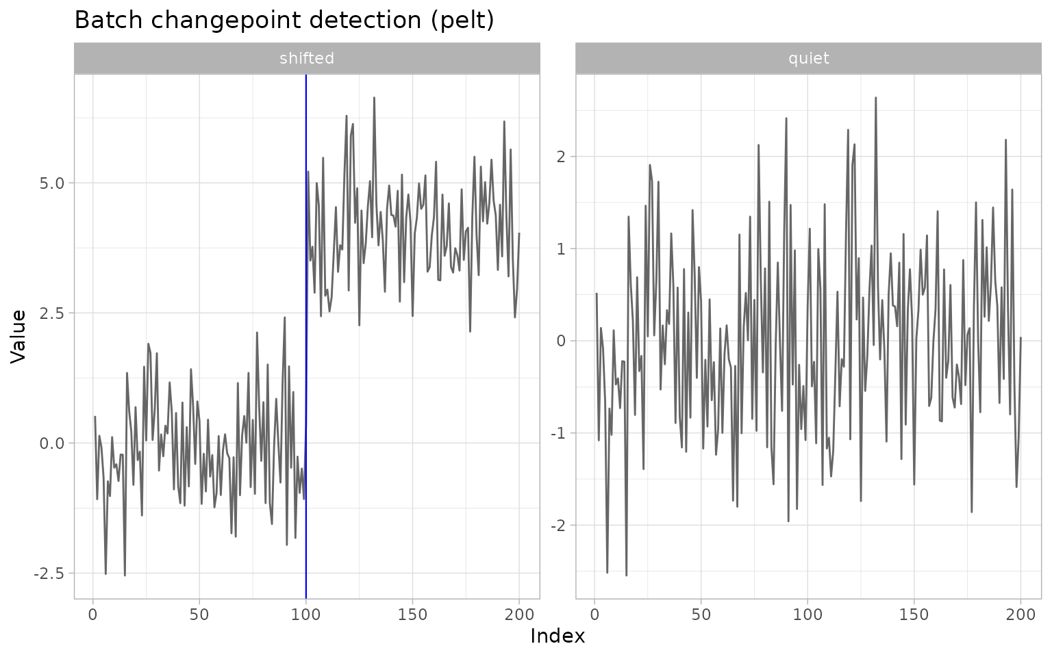

Stability diagnostics

Most engines report a point set with no measure of its fragility. cpt_stability() resamples residuals within the fitted segments — so the estimated regime structure is preserved — re-runs the detector on each replicate, and reports how often each location is re-detected: a cheap, model-agnostic confidence signal available for every engine, including the many that ship no intervals of their own:

st <- cpt_stability(x_mean, method = "pelt", B = 50, seed = 1)
st
#> ggcpt_stability (50 bootstrap replicates, method: pelt)
#> 
#> Original changepoints and their re-detection frequency:
#> # A tibble: 1 × 2
#>      cp stability
#>   <int>     <dbl>
#> 1   100         1
autoplot(st)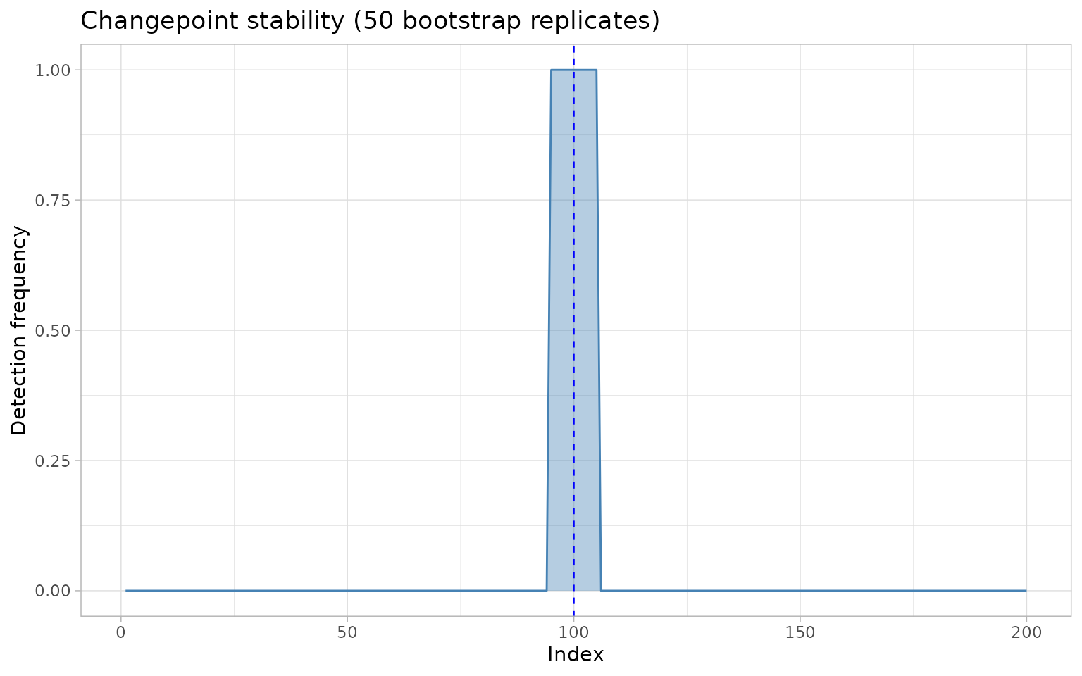

Evaluation, interactivity, and citations

When ground truth is known, cpt_metrics() computes precision, recall and F1 under one-to-one matching, the covering metric, Hausdorff distance, and adjusted Rand index, following the conventions of the modern benchmarking literature (van den Burg and Williams 2020); ggcpt_eval() draws the agreement, and ggcpt_compare() juxtaposes methods. These are the subject of the companion vignette vignette("comparison", package = "ggchangepoint").

Any result renders as an interactive HTML widget with ggcpt_interactive(res) (engine plotly, in Suggests); the static autoplot() path is untouched.

Finally, because every method here is someone’s published work, cpt_cite() returns the reference(s) behind a result, so analyses can cite the right paper without leaving R:

cpt_cite("pelt")
#> [pelt] Killick, R., Fearnhead, P. and Eckley, I. A. (2012). Optimal detection of changepoints with a linear computational cost. Journal of the American Statistical Association, 107(500), 1590-1598.

Discussion

ggchangepoint does not contribute a new detection algorithm; it contributes a surface. The value of a common contract compounds with the number of methods behind it: the same tidy() pipeline, the same plot, and the same evaluation code now span penalised, multiscale, nonparametric, Bayesian, high-dimensional, and regression-based detection — 31 methods in this release. Four more, whose engines are not currently on CRAN (graph-constrained gfpop (Hocking et al. 2020), robust segmentation under outliers (Fearnhead and Rigaill 2019), FOCuS, and sparsified binary segmentation), are listed as planned in cpt_methods() and will slot into the same wrapper pattern once their engines return; until then they are not callable.

Two practical notes. First, wrapped engines run with sensible defaults, but every wrapper forwards ... to its engine and the raw fit is always in $fit — the package is a front door, not a cage. Second, detection quality belongs to the engines; the package’s own additions (metrics, stability, penalty paths) are deliberately engine-agnostic, so conclusions drawn with them transfer between methods.

Acknowledgements

This package stands on the shoulders of the authors of the wrapped engines and of the R (R Core Team 2024), ggplot2 (Wickham 2016), and broom (Robinson 2017) projects.

References

Adams, Ryan Prescott, and David JC MacKay. 2007. “Bayesian Online Changepoint Detection.” arXiv Preprint arXiv:0710.3742.

Aminikhanghahi, Samaneh, and Diane J Cook. 2017. “A Survey of Methods for Time Series Change Point Detection.” Knowledge and Information Systems 51 (2): 339–67. https://doi.org/10.1007/s10115-016-0987-z.

Anastasiou, Andreas, and Piotr Fryzlewicz. 2022. “Detecting Multiple Generalized Change-Points by Isolating Single Ones.” Metrika 85: 141–74. https://doi.org/10.1007/s00184-021-00821-6.

Arlot, Sylvain, Alain Celisse, and Zaid Harchaoui. 2019. “A Kernel Multiple Change-Point Algorithm via Model Selection.” Journal of Machine Learning Research 20 (162): 1–56.

Athey, Susan, Mohsen Bayati, Guido Imbens, and Zhaonan Qu. 2022. “Detecting Change Points in High-Dimensional Time Series.” Journal of Econometrics 227 (2): 367–89.

Bai, Jushan, and Pierre Perron. 1998. “Estimating and Testing Linear Models with Multiple Structural Changes.” Econometrica 66 (1): 47–78.

Bai, Jushan, and Pierre Perron. 2003. “Computation and Analysis of Multiple Structural Change Models.” Journal of Applied Econometrics 18 (1): 1–22.

Baranowski, Rafał, Yining Chen, and Piotr Fryzlewicz. 2019. “Narrowest-over-Threshold Detection of Multiple Change Points and Change-Point-Like Features.” Journal of the Royal Statistical Society Series B 81 (3): 649–72. https://doi.org/10.1111/rssb.12322.

Barry, Daniel, and John A Hartigan. 1993. “A Bayesian Analysis for Change Point Problems.” Journal of the American Statistical Association 88 (421): 309–19.

Beaulieu, Claudie, and Rebecca Killick. 2018. “Distinguishing Trends and Shifts from Memory in Climate Data.” Journal of Climate 31 (23): 9519–43.

Cabrieto, Jedelyn, Janne Adolf, Francis Tuerlinckx, Peter Kuppens, and Eva Ceulemans. 2018. “Detecting Long-Lived Autodependency Changes in a Multivariate System via Change Point Detection and Regime Switching Models.” Scientific Reports 8: 15637.

Chen, Yudong, Tengyao Wang, and Richard J Samworth. 2022. “High-Dimensional, Multiscale Online Changepoint Detection.” Journal of the Royal Statistical Society: Series B 84 (1): 234–66.

Donoho, David L, and John M Johnstone. 1994. “Ideal Spatial Adaptation by Wavelet Shrinkage.” Biometrika 81 (3): 425–55. https://doi.org/10.1093/biomet/81.3.425.

Eichinger, Birte, and Claudia Kirch. 2018. “A MOSUM Procedure for the Estimation of Multiple Random Change Points.” Bernoulli 24 (1): 526–64. https://doi.org/10.3150/16-BEJ887.

Erdman, Chandra, and John W Emerson. 2007. “Bcp: An r Package for Performing a Bayesian Analysis of Change Point Problems.” Journal of Statistical Software 23 (3): 1–13.

Fearnhead, Paul, and Daniel Grose. 2024. “Cpop: Detecting Changes in Piecewise-Linear Signals.” Journal of Statistical Software 109 (7): 1–30.

Fearnhead, Paul, Robert Maidstone, and Adam Letchford. 2019. “Detecting Changes in Slope with an L0 Penalty.” Journal of Computational and Graphical Statistics 28 (2): 265–75.

Fearnhead, Paul, and Guillem Rigaill. 2019. “Changepoint Detection in the Presence of Outliers.” Journal of the American Statistical Association 114 (525): 169–83. https://doi.org/10.1080/01621459.2017.1385466.

Frick, Klaus, Axel Munk, and Hannes Sieling. 2014. “Multiscale Change Point Inference.” Journal of the Royal Statistical Society: Series B 76 (3): 495–580.

Fryzlewicz, Piotr. 2014. “Wild Binary Segmentation for Multiple Change-Point Detection.” The Annals of Statistics 42 (6): 2243–81. https://doi.org/10.1214/14-AOS1245.

Fryzlewicz, Piotr. 2020. “Detecting Multiple Change-Point Features via Narrowest-over-Threshold.” Journal of the Royal Statistical Society Series B 82 (5): 1377–418.

Fryzlewicz, Piotr. 2022. “Tail-Greedy Bottom-up Data Decompositions and Fast Multiple Change-Point Detection.” The Annals of Statistics 50 (5): 2721–61.

Grundy, Thomas, Rebecca Killick, and Gueorgui Mihaylov. 2020. “High-Dimensional Changepoint Detection via a Geometrically Inspired Mapping.” Statistics and Computing 30: 1155–66.

Haslett, John, and Adrian E Raftery. 1989. “Space-Time Modelling with Long-Memory Dependence: Assessing Ireland’s Wind Power Resource.” Journal of the Royal Statistical Society: Series C 38 (1): 1–21.

Haynes, Kaylea, Paul Fearnhead, and Idris A Eckley. 2017. “A Computationally Efficient Nonparametric Approach for Changepoint Detection.” Statistics and Computing 27 (5): 1313–29. https://doi.org/10.1007/s11222-016-9687-5.

Hocking, Toby Dylan, Guillem Rigaill, Paul Fearnhead, and Guillaume Bourque. 2020. “Gfpop: An R Package for Unsupervised Graph-Constrained Change-Point Detection.” Journal of Statistical Software 95 (1): 1–30.

James, Nicholas A, and David S Matteson. 2014. “Ecp: An R Package for Nonparametric Multiple Change Point Analysis of Multivariate Data.” Journal of Statistical Software 62 (7): 1–25. https://doi.org/10.18637/jss.v062.i07.

Killick, Rebecca, and Idris Eckley. 2014. “Changepoint: An R Package for Changepoint Analysis.” Journal of Statistical Software 58 (3): 1–19. https://doi.org/10.18637/jss.v058.i03.

Killick, Rebecca, Paul Fearnhead, and Idris A Eckley. 2012. “Optimal Detection of Changepoints with a Linear Computational Cost.” Journal of the American Statistical Association 107 (500): 1590–98. https://doi.org/10.1080/01621459.2012.737745.

Lavielle, Marc. 2005. “Using the Maximum of the CUSUM Statistic to Detect Changes.” Computational Statistics & Data Analysis 48 (4): 679–96.

Li, Xingchi, and Xianyang Zhang. 2024. “Fastcpd: Fast Change Point Detection in r.” arXiv Preprint arXiv:2404.05933.

Maidstone, Robert, Toby Hocking, Guillem Rigaill, and Paul Fearnhead. 2017. “On Optimal Multiple Changepoint Algorithms for Large Data.” Statistics and Computing 27 (2): 519–33. https://doi.org/10.1007/s11222-016-9636-3.

Matteson, David S, and Nicholas A James. 2014. “A Nonparametric Approach for Multiple Change Point Analysis of Multivariate Data.” Journal of the American Statistical Association 109 (505): 334–45.

McGonigle, Euan T, and Haeran Cho. 2025. “Nonparametric Data Segmentation in Multivariate Time Series via Joint Characteristic Functions.” Biometrika 112 (2): asaf024.

Muggeo, Vito MR. 2003. “Estimating Regression Models with Unknown Break-Points.” Statistics in Medicine 22 (19): 3055–71.

Muggeo, Vito MR. 2008. “Segmented: An r Package to Fit Regression Models with Broken-Line Relationships.” R News 8 (1): 20–25.

Page, Ewan S. 1954. “Continuous Inspection Schemes.” Biometrika 41 (1/2): 100–115.

Pein, Florian, Hannes Sieling, and Axel Munk. 2017. “Heterogeneous Change Point Inference.” Journal of the Royal Statistical Society: Series B 79 (4): 1207–27.

Picard, Franck, Stéphane Robin, Marc Lavielle, Christiane Vaisse, and Jean-Jacques Daudin. 2005. “A Statistical Approach for Array CGH Data Analysis.” BMC Bioinformatics 6 (1): 27.

R Core Team. 2024. R: A Language and Environment for Statistical Computing. R Foundation for Statistical Computing. https://www.R-project.org/.

Robinson, David. 2017. “Broom: An R Package for Converting Statistical Analysis Objects into Tidy Data Frames.” Journal of Open Source Software 2 (19): 401. https://doi.org/10.21105/joss.00401.

Romano, Gaetano, Guillem Rigaill, Vincent Runge, and Paul Fearnhead. 2022. “Detecting Abrupt Changes in the Presence of Local Fluctuations and Autocorrelated Noise.” Journal of the American Statistical Association 117 (540): 2147–62.

Ross, Gordon J. 2015. “Parametric and Nonparametric Sequential Change Detection in r: The Cpm Package.” Journal of Statistical Software 66 (3): 1–20.

Scott, A J, and M Knott. 1974. “A Cluster Analysis Method for Grouping Means in the Analysis of Variance.” Biometrics 30 (3): 507–12.

Truong, Charles, Laurent Oudre, and Nicolas Vayatis. 2020. “Selective Review of Offline Change Point Detection Methods.” Signal Processing 167: 107299. https://doi.org/10.1016/j.sigpro.2019.107299.

van den Burg, Gerrit J J, and Christopher K I Williams. 2020. “An Evaluation of Change Point Detection Algorithms.” arXiv Preprint arXiv:2003.06222, ahead of print. https://doi.org/10.48550/arXiv.2003.06222.

Vostrikova, L Ju. 1981. “Detecting ‘Disorder’ in Multidimensional Random Processes.” Soviet Mathematics Doklady 24: 55–59.

Wang, Tengyao, and Richard J Samworth. 2018. “High Dimensional Change Point Estimation via Sparse Projection.” Journal of the Royal Statistical Society: Series B 80 (1): 57–83.

Wickham, Hadley. 2016. Ggplot2: Elegant Graphics for Data Analysis. Springer. https://doi.org/10.1007/978-3-319-24277-4.

Yao, Yi-Ching. 1988. “Estimating the Number of Change-Points via Schwarz’ Criterion.” Statistics & Probability Letters 6 (3): 181–89. https://doi.org/10.1016/0167-7152(88)90118-6.

Zeileis, Achim, Friedrich Leisch, Kurt Hornik, and Christian Kleiber. 2002. “Strucchange: An r Package for Testing for Structural Change in Linear Regression Models.” Journal of Statistical Software 7 (2): 1–38.

Zhao, Kaiguang, Michael A Wulder, Tongxi Hu, et al. 2019. “Detecting Change-Point, Trend, and Seasonality in Satellite Time Series Data to Track Abrupt Changes and Nonlinear Dynamics: A Bayesian Ensemble Algorithm.” Remote Sensing of Environment 232: 111181.

Zhao, Zifeng, Feiyu Jiang, and Xiaofeng Shao. 2022. “Segmenting Time Series via Self-Normalisation.” Journal of the Royal Statistical Society: Series B 84 (5): 1699–725.