Comparing and Evaluating Changepoint Methods with ggchangepoint

Youzhi Yu
University of Chicago

Abstract

No single changepoint detection method dominates across signal shapes, noise regimes, and computational budgets: large-scale evaluations find that the ranking of algorithms is highly dataset-dependent and that default configurations are often far from optimal (van den Burg and Williams 2020; Truong et al. 2020). Sound practice therefore requires running several detectors, comparing their outputs, and — when ground truth is available — scoring them with well-defined accuracy metrics. This article presents the comparison and evaluation toolkit of ggchangepoint: visual comparison across methods (ggcpt_compare()), a common tidy representation of competing segmentations (ggcpt_compare_table()), a metrics module implementing precision/recall/F1 under one-to-one matching, the covering metric, Hausdorff distance, and the adjusted Rand index (cpt_metrics()), multi-annotator scoring in the style of the Turing Change Point Dataset benchmark (cpt_metrics_annotated()), and visual evaluation against ground truth (ggcpt_eval()). We further discuss three complementary tools for quantifying the uncertainty of a segmentation — engine-native confidence intervals, bootstrap stability profiles (cpt_stability()), and the CROPS penalty path (cpt_crops()) — and close with a small simulation-based benchmarking workflow built from the package’s ground-truth generators.

Introduction

The changepoint literature offers a wide menu of detectors — penalised optimal partitioning, binary segmentation and its wild and narrowest-over-threshold refinements, moving-sum statistics, nonparametric divergence measures, Bayesian posteriors — each with its own inductive bias (Aminikhanghahi and Cook 2017; Truong et al. 2020). Benchmarks that score many algorithms on many series find no uniform winner: performance depends on the kind of change (mean, variance, distribution), the noise (Gaussian, heavy-tailed, autocorrelated), the number and spacing of changes, and the tuning of penalties and thresholds (van den Burg and Williams 2020). Two practical consequences follow. First, an analyst should compare several methods on the data at hand rather than trust one default. Second, when ground truth (or expert annotation) exists, comparison should be quantitative, using metrics with agreed conventions.

ggchangepoint supports both activities behind one interface. Every detector returns the same tidy ggcpt object, so competing methods are directly comparable; the comparison module renders them side by side, and the evaluation module scores them. This article is the package’s methods-paper treatment of that workflow. The companion vignette vignette("introduction", package = "ggchangepoint") documents the full detection surface; here we take detectors as given and focus on comparison, evaluation, and uncertainty.

Problem setup

Let $y_{1:n} = (y_1, \dots, y_n)$ be an ordered sequence. A segmentation with $m$ changepoints is an ordered set $\tau_{0:m+1}$ with $0 = \tau_0 < \tau_1 < \cdots < \tau_m < \tau_{m+1} = n$, partitioning the index set into segments $A_j = \{\tau_{j-1}+1, \dots, \tau_j\}$, $j = 1, \dots, m+1$. Most offline methods minimise a penalised cost $$\sum_{j=1}^{m+1} \mathcal{C}\bigl(y_{(\tau_{j-1}+1):\tau_j}\bigr) + \beta f(m),$$ where $\mathcal{C}(\cdot)$ is a segment cost and $\beta f(m)$ guards against over-segmentation (Yao 1988; Killick et al. 2012).

Throughout the package a changepoint $\tau$ is reported in the “left” convention: $\tau$ is the last index of the left segment, the convention of the changepoint package (Killick et al. 2012). Engines that natively report the first index of the right segment (e.g. the ecp family, Matteson and James (2014)) are normalised on the way in, so comparisons across methods are always like for like.

Comparing segmentations is harder than comparing point estimates for three reasons. First, the number of detected changes varies across methods, so a metric must handle unequal-length sets. Second, a detection a few indices away from a true change is usually acceptable, so metrics need a tolerance margin — and a matching rule that prevents one true change from being “claimed” by several detections. Third, changepoint sets induce partitions, and two very different-looking point sets can induce similar partitions; good practice therefore reports both point-based metrics (precision/recall, Hausdorff) and partition-based metrics (covering, Rand) (van den Burg and Williams 2020).

Visual comparison

We simulate a series with three mean levels (two changepoints) and run several detectors through the unified dispatcher. ggcpt_compare() accepts the raw series and a vector of method names, runs cpt_detect() for each, and renders the results. The default layout = "facet" draws one panel per method:

set.seed(2024)
x <- c(rnorm(150, 0), rnorm(150, 3), rnorm(200, 1))
ggcpt_compare(x, methods = cmp_methods)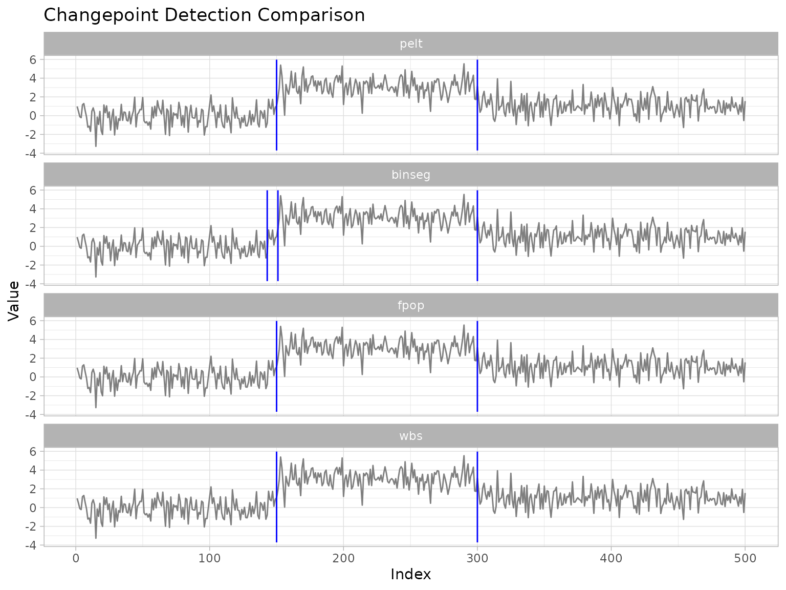

A method that finds no changepoints keeps its panel — ruleless, but present — rather than silently disappearing. A method that ran and found nothing is a result, not a missing value:

set.seed(7)
x_null <- rnorm(300)
ggcpt_compare(x_null, methods = c("pelt", "binseg"))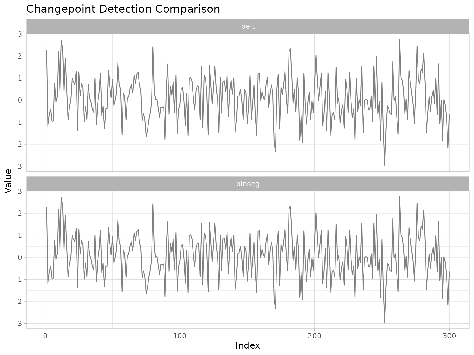

The layout = "overlay" variant superimposes all methods in a single panel with colour-coded rules, which makes both kinds of disagreement easier to see: small differences in an estimated location, and outright differences in how many changepoints a method reports.

ggcpt_compare(x, methods = cmp_methods, layout = "overlay")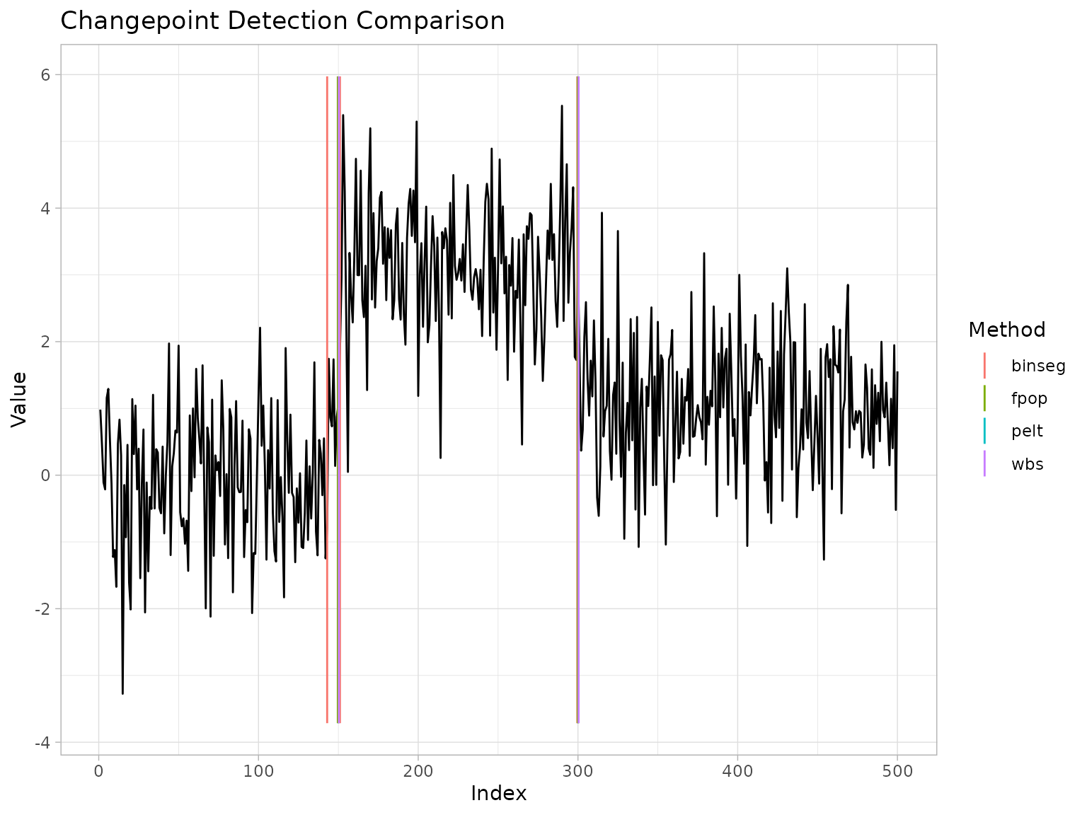

For a numeric rather than visual comparison, ggcpt_compare_table() returns one tidy tibble with a row per (method, changepoint) pair; a method that found nothing contributes a single row with cp = NA, which is the table’s version of keeping the empty panel:

ggcpt_compare_table(x, methods = cmp_methods)
#> # A tibble: 9 × 3
#>   method    cp cp_value
#>   <chr>  <int>    <dbl>
#> 1 pelt     150    1.05 
#> 2 pelt     300    3.14 
#> 3 binseg   143   -0.796
#> 4 binseg   151    1.86 
#> 5 binseg   300    3.14 
#> 6 fpop     150    1.05 
#> 7 fpop     300    3.14 
#> 8 wbs      150    1.05 
#> 9 wbs      300    3.14

Because every row carries the same columns, this table pipes directly into dplyr/ggplot2 summaries — counting detections per method, plotting location agreement, and so on (Wickham 2016). When the detectors are slow, ggcpt_compare() honours future::plan() (through future.apply) and fits them in parallel.

Accuracy metrics

When the true changepoints $\mathcal{T} = \{t_1, \dots, t_K\}$ are known, cpt_metrics(pred, truth, n, margin) scores a predicted set $\mathcal{P} = \{p_1, \dots, p_M\}$ with the following quantities.

Precision, recall, and F1 under one-to-one matching. A prediction $p$matches a truth $t$ if $|p - t| \le \texttt{margin}$. Matching is one-to-one: predictions are scanned in increasing order and each takes the earliest unmatched truth within the margin, so each truth is claimed by at most one prediction (for points on a line this greedy rule attains a maximum matching). With $\mathrm{TP}$ matched pairs, $$\mathrm{precision} = \frac{\mathrm{TP}}{|\mathcal{P}|}, \qquad \mathrm{recall} = \frac{\mathrm{TP}}{|\mathcal{T}|}, \qquad F_1 = \frac{2\,\mathrm{precision}\cdot\mathrm{recall}} {\mathrm{precision} + \mathrm{recall}},$$ with $F_1 = 0$ by convention when precision and recall are both zero. Because $\mathrm{TP}$ counts pairs, all three quantities lie in $[0, 1]$: three predictions crowded around one true change score one true positive, not three.

The covering metric. Following van den Burg and Williams (2020), let $\mathcal{S}$ and $\mathcal{S}'$ be the partitions induced by the truth and the prediction, and $J(A, A') = |A \cap A'| / |A \cup A'|$ the Jaccard index of two segments. The covering of $\mathcal{S}$ by $\mathcal{S}'$ is $$\mathrm{cov}(\mathcal{S}, \mathcal{S}') = \frac{1}{n} \sum_{A \in \mathcal{S}} |A| \, \max_{A' \in \mathcal{S}'} J(A, A'),$$ a weighted average of the best overlap achieved for each true segment.

Hausdorff distance. The worst-case location error, in index units, $\max\{\max_p \min_t |p - t|,\; \max_t \min_p |p - t|\}$; it is NA when either set is empty, since there is no distance to a nonexistent point.

Adjusted Rand index. The chance-corrected agreement of the two induced segment labellings; 1 for identical partitions, 0 for chance-level agreement.

Annotation error and matched location errors. The absolute difference in counts $\bigl||\mathcal{P}| - |\mathcal{T}|\bigr|$, and the MAE/RMSE of the matched location pairs — the latter two NA when nothing matched, because an average over no pairs is not zero error.

# perfect detection
cpt_metrics(pred = c(150, 300), truth = c(150, 300), n = 500)
#> # A tibble: 1 × 12
#>       n n_pred n_truth precision recall    f1 covering hausdorff rand_index
#>   <int>  <int>   <int>     <dbl>  <dbl> <dbl>    <dbl>     <dbl>      <dbl>
#> 1   500      2       2         1      1     1        1         0          1
#> # ℹ 3 more variables: annotation_error <int>, mae_matched <dbl>,
#> #   rmse_matched <dbl>

# near misses within the margin still match one-to-one
cpt_metrics(pred = c(148, 305), truth = c(150, 300), n = 500, margin = 5)
#> # A tibble: 1 × 12
#>       n n_pred n_truth precision recall    f1 covering hausdorff rand_index
#>   <int>  <int>   <int>     <dbl>  <dbl> <dbl>    <dbl>     <dbl>      <dbl>
#> 1   500      2       2         1      1     1    0.973         5      0.958
#> # ℹ 3 more variables: annotation_error <int>, mae_matched <dbl>,
#> #   rmse_matched <dbl>

# three predictions around one truth: one TP, precision 1/3
cpt_metrics(pred = c(148, 150, 152), truth = c(150), n = 500, margin = 5)
#> # A tibble: 1 × 12
#>       n n_pred n_truth precision recall    f1 covering hausdorff rand_index
#>   <int>  <int>   <int>     <dbl>  <dbl> <dbl>    <dbl>     <dbl>      <dbl>
#> 1   500      3       1     0.333      1   0.5    0.992         2      0.984
#> # ℹ 3 more variables: annotation_error <int>, mae_matched <dbl>,
#> #   rmse_matched <dbl>

Three edge-case conventions deserve emphasis, because getting them wrong silently corrupts benchmark averages:

• Both sets empty. Predicting “no changepoints” for a series with no changepoints is exactly right, so precision, recall, F1, covering, and the Rand index all equal 1. (Hausdorff distance and the matched-location errors remain NA: there are no pairs to measure.)
• Empty prediction, non-empty truth. An empty changepoint set still induces a perfectly well-defined partition — the trivial one with a single segment — so covering scores it by segment overlap rather than awarding an automatic 0. Precision and recall are 0, and the adjusted Rand index is 0 because the trivial partition agrees with the truth only at chance level.
• Out-of-range indices. Changepoint locations must lie in $\{1, \dots, n-1\}$ under the left convention; anything outside is dropped with a warning rather than corrupting the partition construction, and the metrics are then computed on what remains.

# a correct "no change" answer is rewarded
cpt_metrics(pred = integer(0), truth = integer(0), n = 300)
#> # A tibble: 1 × 12
#>       n n_pred n_truth precision recall    f1 covering hausdorff rand_index
#>   <int>  <int>   <int>     <dbl>  <dbl> <dbl>    <dbl>     <dbl>      <dbl>
#> 1   300      0       0         1      1     1        1        NA          1
#> # ℹ 3 more variables: annotation_error <int>, mae_matched <dbl>,
#> #   rmse_matched <dbl>

# empty prediction against one true change at the midpoint: the trivial
# one-segment partition still overlaps half the series, so covering is 0.5
cpt_metrics(pred = integer(0), truth = c(150), n = 300)
#> # A tibble: 1 × 12
#>       n n_pred n_truth precision recall    f1 covering hausdorff rand_index
#>   <int>  <int>   <int>     <dbl>  <dbl> <dbl>    <dbl>     <dbl>      <dbl>
#> 1   300      0       1         0      0     0      0.5        NA          0
#> # ℹ 3 more variables: annotation_error <int>, mae_matched <dbl>,
#> #   rmse_matched <dbl>

# index 700 cannot be a changepoint of a length-500 series
cpt_metrics(pred = c(100, 700), truth = c(100, 300), n = 500)
#> Warning: Dropping changepoint indices outside 1..(n-1): 700
#> # A tibble: 1 × 12
#>       n n_pred n_truth precision recall    f1 covering hausdorff rand_index
#>   <int>  <int>   <int>     <dbl>  <dbl> <dbl>    <dbl>     <dbl>      <dbl>
#> 1   500      1       2         1    0.5 0.667      0.6       200      0.418
#> # ℹ 3 more variables: annotation_error <int>, mae_matched <dbl>,
#> #   rmse_matched <dbl>

Multi-annotator evaluation

For real data, “ground truth” is often a set of human annotations that disagree with one another. The Turing Change Point Dataset benchmark (van den Burg and Williams 2020) therefore scores a prediction against each annotator and averages. cpt_metrics_annotated() implements this convention: it takes a list of annotation vectors and returns the averaged precision, recall, F1, and covering.

annotations <- list(
  ann1 = c(150, 300),
  ann2 = c(152, 301),
  ann3 = c(149)          # a third annotator missed the second change
)
cpt_metrics_annotated(pred = c(150, 300), annotations, n = 500, margin = 5)
#> # A tibble: 1 × 7
#>       n n_annotators n_pred precision recall    f1 covering
#>   <dbl>        <int>  <int>     <dbl>  <dbl> <dbl>    <dbl>
#> 1   500            3      2     0.833      1 0.889    0.895

Averaging per annotator rather than pooling the annotations matters. The prediction matches both of the first two annotators completely; against the third it finds the one change that annotator marked but also reports a second one, scoring precision $1/2$ and recall $1$. The averages are therefore precision $5/6$ and recall $1$: the disagreement is charged to precision, which is the honest place for it, since the extra detection may well be real and merely unannotated.

Visual evaluation

ggcpt_eval() overlays predictions and ground truth on the series, shades the tolerance window around each true change, and colours each prediction as a true positive or false positive, with missed truths drawn as dashed “Miss” rules. It uses the same one-to-one matching as cpt_metrics(), so the picture and the numbers always agree:

truth <- c(150, 300)
pred <- c(151, 240)      # one hit, one false alarm, one miss
ggcpt_eval(pred, truth, data_vec = x, margin = 5)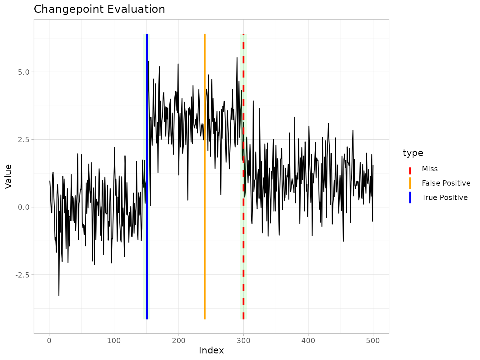

cpt_metrics(pred, truth, n = length(x), margin = 5)
#> # A tibble: 1 × 12
#>       n n_pred n_truth precision recall    f1 covering hausdorff rand_index
#>   <int>  <int>   <int>     <dbl>  <dbl> <dbl>    <dbl>     <dbl>      <dbl>
#> 1   500      2       2       0.5    0.5   0.5    0.784        60      0.696
#> # ℹ 3 more variables: annotation_error <int>, mae_matched <dbl>,
#> #   rmse_matched <dbl>

One true positive out of two predictions and two truths gives precision, recall, and F1 all equal to $0.5$ — the single blue rule, the single orange rule, and the single dashed rule in the plot, counted.

Uncertainty beyond point sets

A segmentation is a point estimate. Three complementary tools quantify how much confidence it deserves.

Engine-native confidence intervals

Some engines deliver genuine confidence statements for changepoint locations. SMUCE (Frick et al. 2014) controls, at level $\alpha$, the probability of overestimating the number of changepoints, and returns a confidence interval for every location; the Bai–Perron dynamic program (Bai and Perron 2003; Zeileis et al. 2002) returns break-date intervals for regression breaks. Four wrapped engines report such intervals — smuce, hsmuce, strucchange, and segmented — as ci_lower/ci_upper columns on the ggcpt changepoints tibble, which autoplot(show_ci = TRUE) draws as whiskers below the series. show_fit = TRUE adds the engine’s own fitted signal, available here and from decafs, cpop, segmented, bcp, and beast:

res_smuce <- smuce_wrapper(x)
tidy(res_smuce)
#> # A tibble: 2 × 4
#>      cp cp_value ci_lower ci_upper
#>   <int>    <dbl>    <int>    <int>
#> 1   150     1.05      146      152
#> 2   300     3.14      295      306
autoplot(res_smuce, show_ci = TRUE, show_fit = TRUE)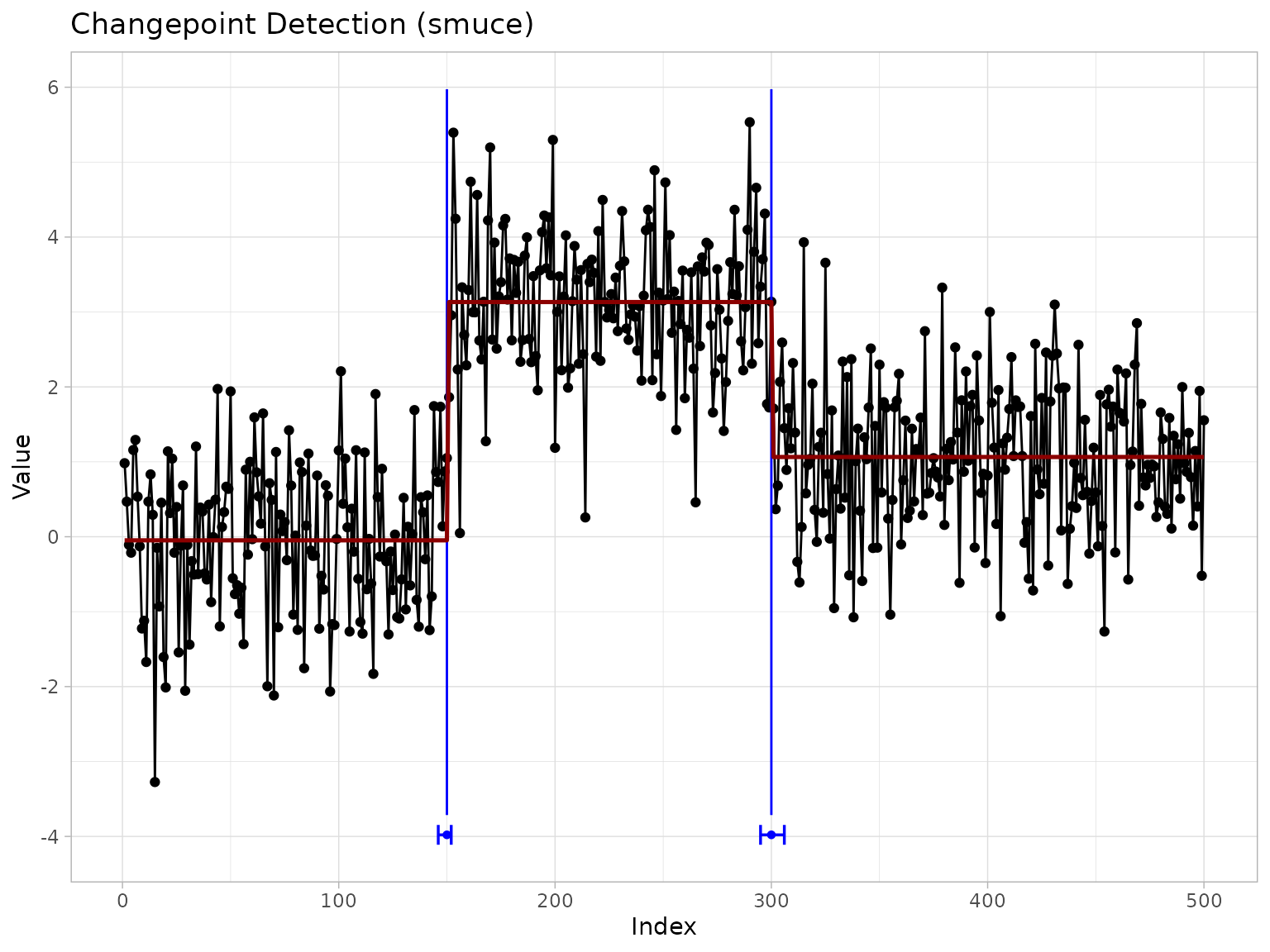

res_bp <- strucchange_wrapper(x)
tidy(res_bp)
#> # A tibble: 2 × 4
#>      cp cp_value ci_lower ci_upper
#>   <int>    <dbl>    <int>    <int>
#> 1   150     1.05      149      152
#> 2   300     3.14      297      303

Such intervals are worth reading alongside each other: two engines can agree on where a change is and still, under their different noise models, disagree about how tightly the location is pinned down.

Bootstrap stability

Most engines ship no intervals at all. cpt_stability() provides a cheap, model-agnostic substitute: it fits the detector once, resamples residuals within the fitted segments (preserving the estimated regime structure), re-runs the detector on each replicate, and reports the proportion of replicates that re-detect a change within margin of each index. Locations that survive resampling are trustworthy; locations that appear in only a fraction of replicates are fragile.

st <- cpt_stability(x, method = "pelt", B = 30, seed = 1)
st
#> ggcpt_stability (30 bootstrap replicates, method: pelt)
#> 
#> Original changepoints and their re-detection frequency:
#> # A tibble: 2 × 2
#>      cp stability
#>   <int>     <dbl>
#> 1   150         1
#> 2   300         1
autoplot(st)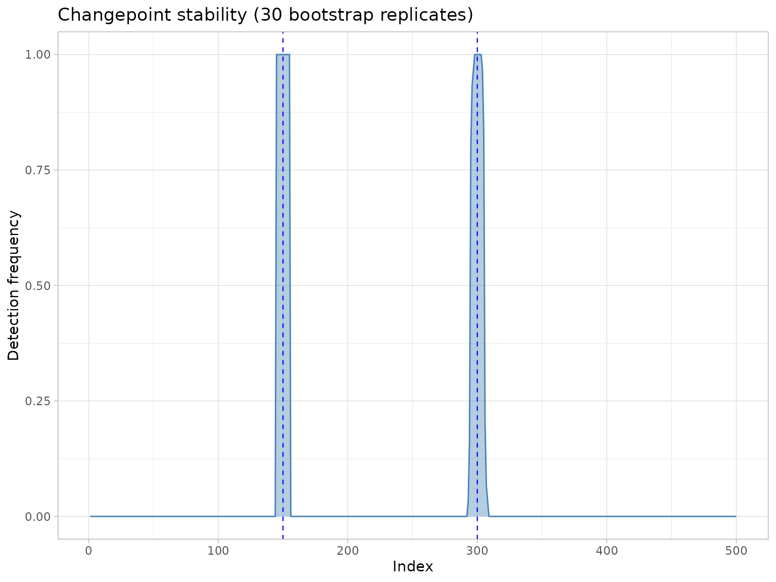

Both changepoints here are re-detected in every replicate, so the point estimate is as stable as this diagnostic can report. The profile is also informative where the print method is silent: a broad, low plateau marks a region the detector keeps splitting somewhere without agreeing where.

Penalty-path sensitivity: CROPS

Penalised methods commit to one penalty $\beta$, and the segmentation can change qualitatively as $\beta$ moves. CROPS (Haynes et al. 2017) computes every optimal segmentation as the penalty ranges over an interval, at roughly one PELT run per distinct solution — penalty selection as a diagnostic rather than a guess. cpt_crops() returns the full path:

path <- cpt_crops(x)
path
#> ggcpt_path (CROPS penalty path)
#>   Change in:       mean 
#>   Penalty range:  [6.215, 62.15]
#>   Series length:   500 
#>   Distinct segmentations: 2 
#> 
#> # A tibble: 2 × 3
#>   penalty n_cpts  cost
#>     <dbl>  <int> <dbl>
#> 1    9.36      2  468.
#> 2    6.21      3  459.

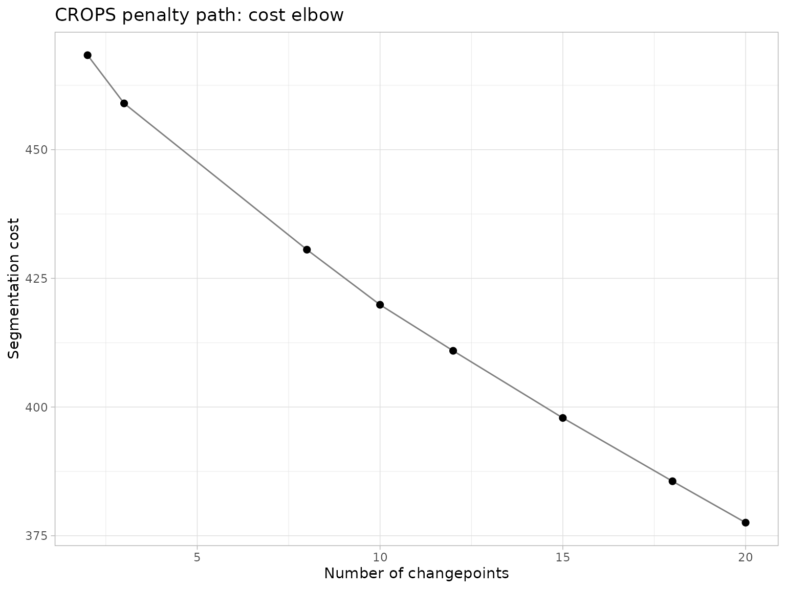
Over the default range $[\log n, 10 \log n]$ this series admits only two distinct segmentations, and the two-changepoint solution holds over all but the very bottom of it. That insensitivity is itself the diagnostic: on a signal this cleanly separated, the answer does not depend on the penalty. Lowering pen_min opens up the rest of the path, where the elbow plot shows the cost reduction per additional changepoint flattening out and the segmentation facets show the candidate models being chosen among:

path_wide <- cpt_crops(x, pen_min = 4)
autoplot(path_wide)                          # cost elbow

autoplot(path_wide, type = "segmentations")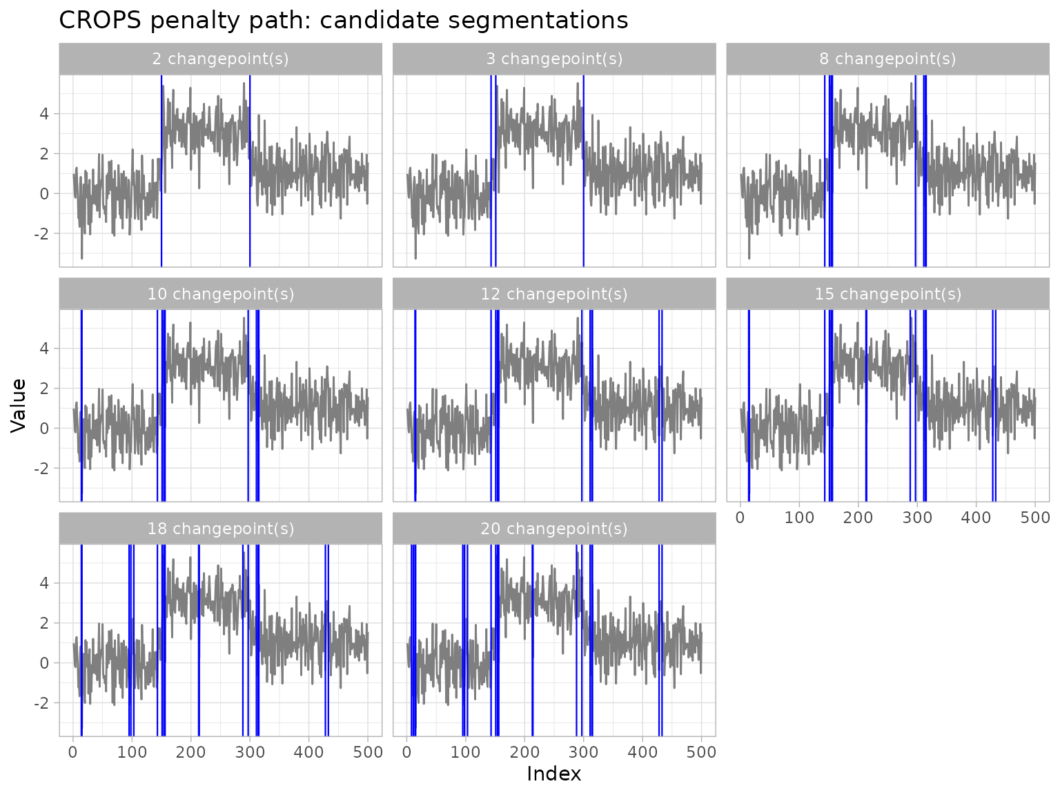

Both cpt_stability() and cpt_crops() operate on a single numeric series and reject multi-column input; for a panel of series, loop over the columns (or use cpt_batch() for the detection step).

A benchmarking workflow

The package’s simulation module closes the loop: generators with known truth feed the metrics module, so methods can be scored over replications. cpt_simulate() draws series with specified changepoints under Gaussian, Student-$t$, AR(1), or random-walk noise, and the canonical test signals of the literature ship as ready-made generators: signal_blocks() (the Donoho–Johnstone blocks signal, Donoho and Johnstone 1994), signal_fms(), signal_mix(), signal_teeth(), and signal_stairs(). Every generator attaches its true changepoints as a true_changepoints attribute, which is exactly the truth argument cpt_metrics() expects.

blocks <- signal_blocks(n = 500, seed = 3)
ggplot(blocks, aes(index, value)) +
  geom_line(colour = "grey40") +
  geom_vline(xintercept = attr(blocks, "true_changepoints"),
             colour = "blue", linewidth = 0.3) +
  labs(title = "signal_blocks(): Donoho-Johnstone blocks with true changepoints")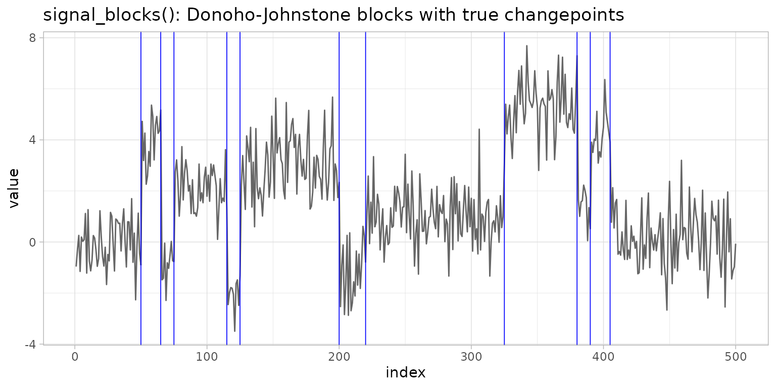

A minimal benchmark: three methods, two signal-to-noise regimes, ten replications each, scored by precision, recall, F1, and covering. The two regimes differ only in the size of the jumps — 2.5 noise standard deviations against 1.0 — so any difference between the panels is attributable to difficulty alone. (Everything stays sequential and small here; cpt_batch() runs one method over many series and honours future::plan() for parallel execution in larger studies.)

methods <- cmp_methods[1:3]
n_rep <- 10
regimes <- list(
  "high SNR (jump 2.5 sd)" = c(0, 2.5, 0.5),
  "low SNR (jump 1.0 sd)"  = c(0, 1.0, 0.3)
)

results <- do.call(rbind, lapply(names(regimes), function(g) {
  do.call(rbind, lapply(seq_len(n_rep), function(r) {
    dat <- cpt_simulate(400, changepoints = c(130, 260), change_in = "mean",
                        params = regimes[[g]], sd = 1, seed = 100 + r)
    truth <- attr(dat, "true_changepoints")
    do.call(rbind, lapply(methods, function(m) {
      fit <- cpt_detect(dat$value, method = m)
      score <- cpt_metrics(fit$changepoints$cp, truth, n = 400, margin = 5)
      cbind(tibble::tibble(regime = g, rep = r, method = m),
            score[, c("precision", "recall", "f1", "covering")])
    }))
  }))
}))

# average over replications, within regime
res_summary <- aggregate(cbind(precision, recall, f1, covering) ~ method + regime,
                         data = results, FUN = mean)
knitr::kable(res_summary, digits = 3,
             caption = "Mean accuracy over 10 replications per regime (margin = 5).")

Mean accuracy over 10 replications per regime (margin = 5).

method	regime	precision	recall	f1	covering
binseg	high SNR (jump 2.5 sd)	0.95	0.95	0.950	0.993
fpop	high SNR (jump 2.5 sd)	0.95	0.95	0.950	0.993
pelt	high SNR (jump 2.5 sd)	0.95	0.95	0.950	0.993
binseg	low SNR (jump 1.0 sd)	0.65	0.60	0.617	0.852
fpop	low SNR (jump 1.0 sd)	0.65	0.65	0.650	0.884
pelt	low SNR (jump 1.0 sd)	0.70	0.65	0.667	0.857

Two regimes are enough to reproduce the claim this article opened with. In the high-SNR panel the problem is close to solved and the methods are hard to tell apart; shrinking the jump to one noise standard deviation lowers all four metrics for every method and opens a visible gap between them, so an ordering read off the easy regime need not survive into the hard one. Accuracy is a property of the (method, signal, noise) triple rather than of the method alone, which is why this loop is worth running on the series at hand instead of adopting a ranking from the literature.

The same skeleton scales to the studies of van den Burg and Williams (2020): more generators (heavy-tailed and autocorrelated noise via cpt_simulate(noise = "t") and noise = "ar1"), more methods (everything in cpt_methods()), more replications, and parallel execution via future::plan(multisession).

Discussion

Comparison and evaluation are not afterthoughts in changepoint analysis; they are how an analyst earns confidence in a segmentation. The design of ggchangepoint’s toolkit follows three principles. First, a common representation makes comparison trivial: because every engine returns the same ggcpt contract in the same location convention, ggcpt_compare() and the metrics module work for all 31 wired methods without special cases. Second, metrics must agree with their pictures: ggcpt_eval() and cpt_metrics() share one matching routine, so a plotted true positive is a counted true positive. Third, uncertainty deserves first-class treatment: engine-native intervals, bootstrap stability, and penalty paths give three independent views of how much a reported changepoint should be trusted, and all three render directly with ggplot2 (Wickham 2016).

For the detection surface itself — the dispatcher, the engine wave, the Bayesian displays, and the multivariate tools — see vignette("introduction", package = "ggchangepoint") and the feature tour in vignette("ggchangepoint", package = "ggchangepoint").

References

Aminikhanghahi, Samaneh, and Diane J Cook. 2017. “A Survey of Methods for Time Series Change Point Detection.” Knowledge and Information Systems 51 (2): 339–67. https://doi.org/10.1007/s10115-016-0987-z.

Bai, Jushan, and Pierre Perron. 2003. “Computation and Analysis of Multiple Structural Change Models.” Journal of Applied Econometrics 18 (1): 1–22.

Donoho, David L, and John M Johnstone. 1994. “Ideal Spatial Adaptation by Wavelet Shrinkage.” Biometrika 81 (3): 425–55. https://doi.org/10.1093/biomet/81.3.425.

Frick, Klaus, Axel Munk, and Hannes Sieling. 2014. “Multiscale Change Point Inference.” Journal of the Royal Statistical Society: Series B 76 (3): 495–580.

Haynes, Kaylea, Paul Fearnhead, and Idris A Eckley. 2017. “A Computationally Efficient Nonparametric Approach for Changepoint Detection.” Statistics and Computing 27 (5): 1313–29. https://doi.org/10.1007/s11222-016-9687-5.

Killick, Rebecca, Paul Fearnhead, and Idris A Eckley. 2012. “Optimal Detection of Changepoints with a Linear Computational Cost.” Journal of the American Statistical Association 107 (500): 1590–98. https://doi.org/10.1080/01621459.2012.737745.

Matteson, David S, and Nicholas A James. 2014. “A Nonparametric Approach for Multiple Change Point Analysis of Multivariate Data.” Journal of the American Statistical Association 109 (505): 334–45.

Truong, Charles, Laurent Oudre, and Nicolas Vayatis. 2020. “Selective Review of Offline Change Point Detection Methods.” Signal Processing 167: 107299. https://doi.org/10.1016/j.sigpro.2019.107299.

van den Burg, Gerrit J J, and Christopher K I Williams. 2020. “An Evaluation of Change Point Detection Algorithms.” arXiv Preprint arXiv:2003.06222, ahead of print. https://doi.org/10.48550/arXiv.2003.06222.

Wickham, Hadley. 2016. Ggplot2: Elegant Graphics for Data Analysis. Springer. https://doi.org/10.1007/978-3-319-24277-4.

Yao, Yi-Ching. 1988. “Estimating the Number of Change-Points via Schwarz’ Criterion.” Statistics & Probability Letters 6 (3): 181–89. https://doi.org/10.1016/0167-7152(88)90118-6.

Zeileis, Achim, Friedrich Leisch, Kurt Hornik, and Christian Kleiber. 2002. “Strucchange: An r Package for Testing for Structural Change in Linear Regression Models.” Journal of Statistical Software 7 (2): 1–38.