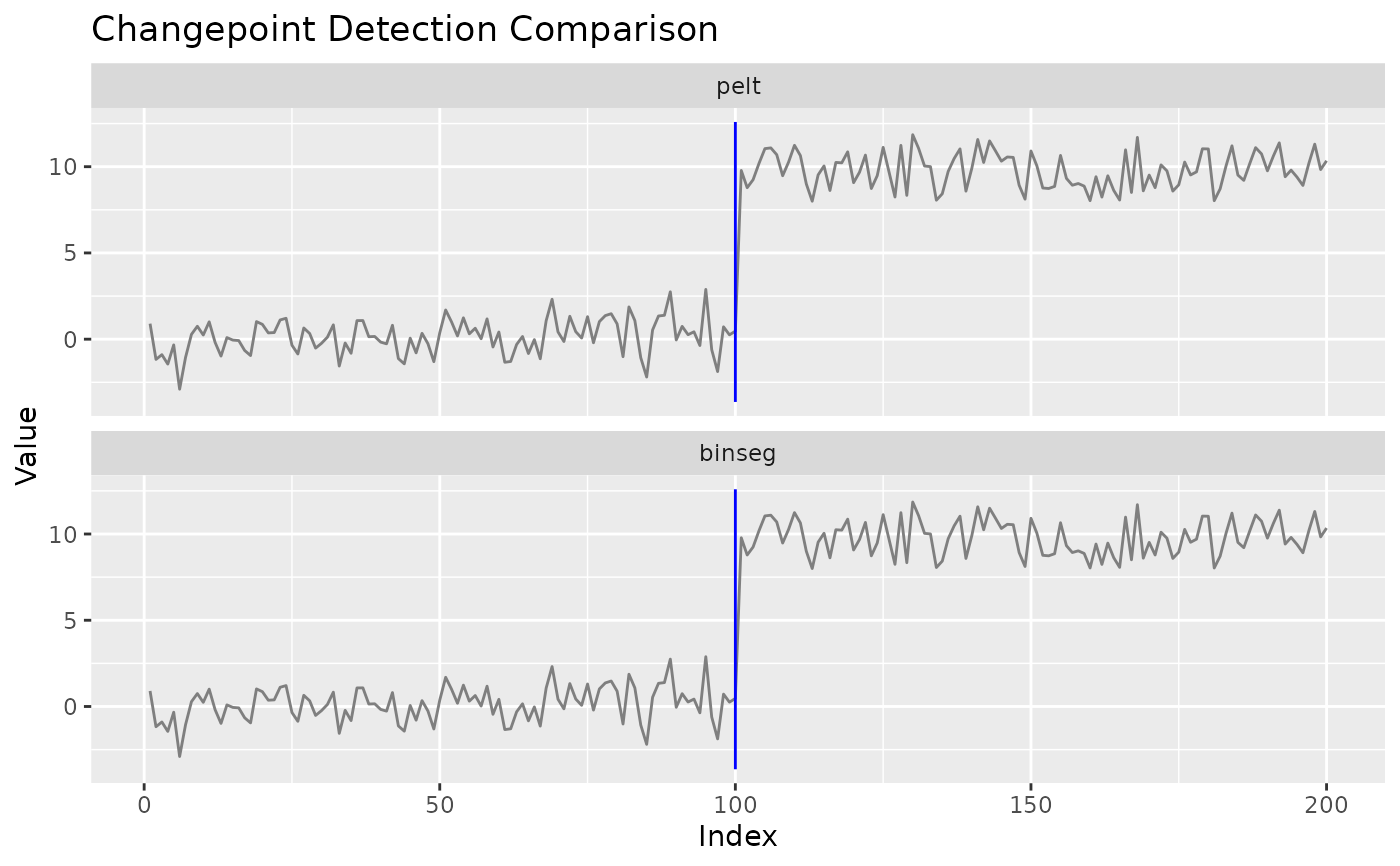
Compare multiple changepoint detection methods — ggcpt

Runs several detectors on the same data and returns a faceted or overlaid ggplot comparison. Respects future::plan() for parallel execution if the future.apply package is available.

Usage

ggcpt_compare(
  x,
  methods = c("pelt", "binseg", "amoc"),
  layout = c("facet", "overlay"),
  change_in = "mean",
  seed = NULL,
  ...
)

Arguments

x: A numeric vector (the data series). A one-column matrix or data frame is accepted; wider input is refused, because these detectors are univariate and flattening the columns would invent a changepoint at every seam. Use cpt_batch() for a panel of series.
methods: Character vector of method names (passed to cpt_detect).
layout: Layout type. "facet" (default) shows one panel per method; "overlay" draws all changepoints in one panel, colour-coded. The overlay dodges the rules horizontally so that two methods agreeing on an index are both visible, which moves each rule by up to half an observation, so read positions off "facet", or off tidy(), and treat the overlay as a picture of agreement rather than of location.
change_in: What to detect change in. Passed to each detector.
seed: Optional seed for reproducible parallelism. Passed to future.apply::future_lapply() as future.seed, and to set.seed() when running sequentially. Left NULL under a parallel plan, future.seed = TRUE is used, so the workers get parallel-safe streams but the run is not reproducible. The seed is scoped to this call: .Random.seed is saved and restored, so a seeded call inside a simulation loop does not pin the loop's own stream.
...: Additional arguments passed to each detector.

Value

A ggplot object.

Positions, not a time index

Unlike cpt_detect(), cpt_batch() and autoplot.ggcpt(), these two take no index: the input is reduced to a bare numeric vector, so a ts, xts, zoo or tsibble is plotted (and tabulated) in observation positions with an "Index" axis. To compare detectors on dated data, run cpt_detect(x, method = m, index = dates) per method and read tidy()'s cp_index, or plot the results with autoplot().

Choosing the method by its answer

Running several methods and reporting the one that found a change, as if it were the only one run, is a garden of forking paths with a plot attached, and fifty methods behind one call make it easier here than anywhere else. A method chosen because of its answer carries no valid p-value, and neither does any test at its changepoints: the selection across methods is a second selection on top of the one each method already makes (see cpt_test()'s selection_adjusted). Choose the method before seeing the data (cpt_recommend() answers from what you know about the problem, not from the series), or report every method you ran. Agreement across methods, as cpt_consensus() counts it, is a robustness display, not a correction: the methods share engines, costs and assumptions.

Examples

set.seed(2022)
x <- c(rnorm(100, 0, 1), rnorm(100, 10, 1))
ggcpt_compare(x, methods = c("pelt", "binseg"))