Significance regions computed in the layer

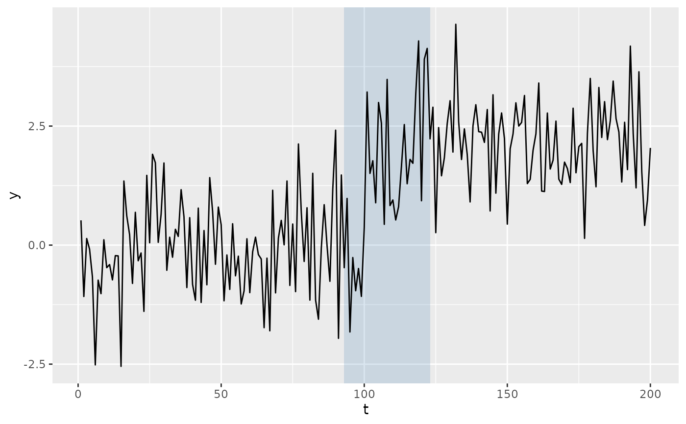
The region twin of stat_changepoint(): runs detection on the layer's own x/y and draws what the method returns as an interval, so ggplot(d, aes(t, y)) + geom_line() + stat_cpt_region() is the whole plot. Narrowest Significance Pursuit (method = "nsp", the default) returns regions, each containing a changepoint at a global significance level; a method with location intervals ("smuce", "strucchange", "segmented", ...) draws those instead.

Usage

stat_cpt_region(
  mapping = NULL,
  data = NULL,
  geom = GeomCptRegion,
  position = "identity",
  ...,
  method = "nsp",
  na.rm = FALSE,
  show.legend = NA
)

Arguments

mapping

Aesthetic mappings.

data

A data frame.

geom

The geom to draw with. Defaults to geom_cpt_region()'s.

position

Position adjustment.

...

Further arguments: those the detector takes (for example alpha for NSP's level, or seed) go to it, the rest to the geom. With method = "nsp" that makes alpha the level, so set the band's transparency through its fill instead (fill = ggplot2::alpha("steelblue", 0.3)).

method

Detection method: "nsp" (the default) or any method whose result carries regions or location intervals (see cpt_methods()$ci).

na.rm

If FALSE, missing values are removed.

show.legend

Whether to show legend.

Value

A ggplot layer.

See also

Other ggplot2 layers: geom_changepoint(), geom_cpt_ci(), geom_cpt_event(), geom_cpt_label(), geom_cpt_region(), geom_cpt_segment(), ggchangepoint-ggproto, stat_changepoint()

Examples

library(ggplot2)
set.seed(2026)
d <- data.frame(t = 1:200, y = c(rnorm(100), rnorm(100, 2)))
ggplot(d, aes(t, y)) + stat_cpt_region(seed = 1) + geom_line()