Inference, Selection and Diagnostics

Youzhi Yu
University of Chicago

Detection gives you locations. This vignette is about the four questions that come next, and that a bare list of locations cannot answer:

1. How sure are we about where? — cpt_confint(), nsp_wrapper().
2. Is the change real at all? — cpt_test(), and why the answer is harder than it looks.
3. How many changes are there? — cpt_select().
4. What is driving this answer? — cpt_influence(), cpt_sensitivity(), cpt_statistic().

set.seed(2026)
x <- c(rnorm(120), rnorm(120, 3), rnorm(120, 0.5))
fit <- cpt_detect(x, method = "pelt")
fit
#> ggcpt (changepoint detection result)
#>   Method:         pelt
#>   Change in:       mean 
#>   Changepoints found: 2 
#>   CP convention:   left 
#>   Penalty:         MBIC 
#>   Series length:   360 
#> 
#> Changepoints:
#> # A tibble: 2 × 2
#>      cp cp_value
#>   <int>    <dbl>
#> 1   120    -1.07
#> 2   240     5.05

1. Where could the changepoint be?

Four provenances, one contract

Only a handful of engines ship an interval of their own. cpt_confint() covers the rest, and — because the four routes mean genuinely different things — reports which one it used in a source column rather than presenting them as interchangeable.

cpt_confint(fit, method = "bootstrap", B = 100, seed = 1)
#> # A tibble: 2 × 6
#>      cp ci_lower ci_upper level source    n_replicates
#>   <int>    <int>    <int> <dbl> <chr>            <int>
#> 1   120      119      120  0.95 bootstrap          100
#> 2   240      238      241  0.95 bootstrap          100

The bootstrap route resamples residuals within the fitted segments, re-runs the detector, and takes quantiles of the re-detected location. It measures the sampling variability of the procedure conditional on the fitted segmentation. It is model-agnostic and available for every engine; it is not exact.

When the engine has its own interval, method = "auto" uses it:

sm <- smuce_wrapper(x)
cpt_confint(sm)
#> # A tibble: 2 × 5
#>      cp ci_lower ci_upper level source
#>   <int>    <int>    <int> <dbl> <chr> 
#> 1   120      117      120    NA native
#> 2   240      239      244    NA native

Those are SMUCE’s simultaneous confidence sets — a different object from a bootstrap frequency band, which is exactly why the source column exists.

A changepoint that is an interval

Narrowest Significance Pursuit (Fryzlewicz 2024) inverts the usual framing. Rather than estimating locations and then asking whether they are real, it returns a set of intervals, each of which contains at least one changepoint, with the guarantee holding globally across all the intervals at level $\alpha$. The coverage is exact and finite-sample.

res_nsp <- nsp_wrapper(x, alpha = 0.1, M = 200, seed = 1)
cpt_regions(res_nsp)
#> # A tibble: 2 × 4
#>   start   end length value
#>   <int> <int>  <int> <dbl>
#> 1   113   122     10  4.31
#> 2   222   253     32  4.47

autoplot(res_nsp)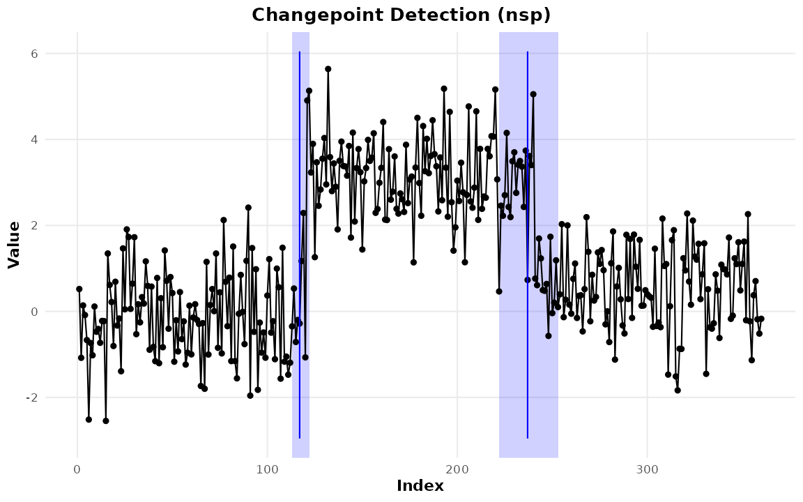

Read the widths. A narrow band is a sharply located change; a wide one is the honest statement that the data pin the change down only loosely. Note what the result does not claim: NSP produces no point estimate, so the cp column holds the interval midpoint, is labelled region_midpoint in cp_source, and says so when the object prints. The region is the inferential object.

The self-normalised and autoregressive variants keep the guarantee under heavy tails, heteroscedasticity and serial dependence:

y_ar <- as.numeric(stats::arima.sim(list(ar = 0.6), 300)) +
  rep(c(0, 3), each = 150)
cpt_regions(nsp_wrapper(y_ar, variant = "ar", ord = 1, M = 200, seed = 1))
#> # A tibble: 0 × 3
#> # ℹ 3 variables: start <int>, end <int>, length <int>

2. Is the change real?

This is where changepoint analysis is most often done wrong. Testing a change at a location that was chosen because the data looked like it changed there is circular, and the resulting p-values are anti-conservative, often severely.

cpt_test() never hides that. It uses the engine’s own test where one exists and an explicitly unadjusted two-sample test where none does, and the selection_adjusted column records which you got:

suppressWarnings(cpt_test(fit))
#> # A tibble: 2 × 6
#>      cp estimate statistic  p_value method                    selection_adjusted
#>   <int>    <dbl>     <dbl>    <dbl> <chr>                     <lgl>             
#> 1   120     3.25      25.6 4.24e-70 Welch two-sample t (unad… FALSE             
#> 2   240    -2.60     -21.7 2.38e-58 Welch two-sample t (unad… FALSE

cpt_test(strucchange_wrapper(x))
#> # A tibble: 2 × 6
#>      cp estimate statistic     p_value method               selection_adjusted
#>   <int>    <dbl>     <dbl>       <dbl> <chr>                <lgl>             
#> 1   120    1.95      149.  0           Chow F (strucchange) TRUE              
#> 2   240   -0.976      28.3 0.000000182 Chow F (strucchange) TRUE

If you need a guarantee that survives selection, the route is NSP (above) or cpt_confint(method = "nsp"), which maps each detected changepoint to the narrowest region covering it and returns NA for one that no region covers — because “no region supports this at level $\alpha$” is a finding, not a missing value.

cpt_confint(fit, method = "nsp", level = 0.9, seed = 1)
#> # A tibble: 2 × 5
#>      cp ci_lower ci_upper level source    
#>   <int>    <int>    <int> <dbl> <chr>     
#> 1   120      113      122   0.9 nsp_region
#> 2   240      222      253   0.9 nsp_region

3. How many changepoints?

cpt_crops() draws the penalty path. cpt_select() chooses from it, over one candidate ladder shared by every criterion — so “BIC says 2, cross-validation says 3” is a comparison of criteria and not of two different searches.

sel <- cpt_select(x, criterion = "mbic", k_max = 8)
sel
#> ggcpt_selection (criterion: mbic, method: pelt)
#>   Candidates scored: K = 0 to 8
#>   Chosen K:          2
#>   Locations:         120, 240
#> 
#> # A tibble: 9 × 4
#>       k  value  cost chosen
#>   <int>  <dbl> <dbl> <lgl> 
#> 1     0 382.   382.  FALSE 
#> 2     1 273.   257.  FALSE 
#> 3     2  -1.55 -33.6 TRUE  
#> 4     3   3.01 -41.5 FALSE 
#> 5     4  11.3  -47.5 FALSE 
#> 6     5  19.4  -54.1 FALSE 
#> 7     6  26.6  -58.5 FALSE 
#> 8     7  33.9  -63.0 FALSE 
#> 9     8  43.1  -67.5 FALSE

criterion = "mbic" is the segment-length modified BIC of Zhang and Siegmund (2007) — the real one, which reads the segment lengths and so cannot be expressed by cpt_penalty()’s function of $n$ and $k$ alone.

autoplot(sel)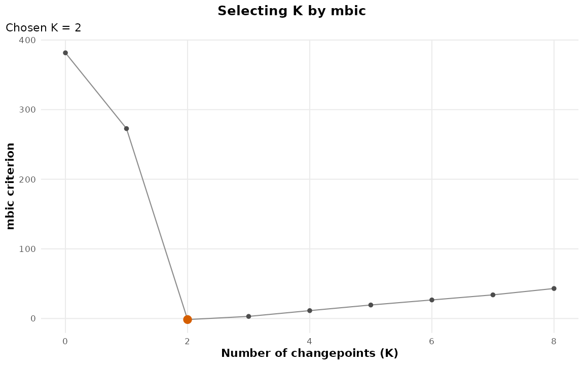

The ladder plot is more informative than the criterion curve, because it shows what each candidate actually is:

autoplot(sel, plot_type = "ladder", max_facets = 6)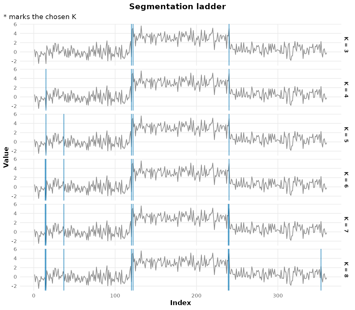

Cross-validation is the criterion with a consistency proof (Zou et al. 2020):

cpt_select(x, criterion = "cv", k_max = 8)$k
#> [1] 2

A note on AIC: its $2k$ penalty does not grow with $n$, so it over-selects and will usually take every rung the ladder offers. It is available because people ask for it and because seeing the curve is instructive, not because it is a good default.

4. What is driving the answer?

Which observation

cpt_stability() answers “would I find this again?”. cpt_influence() asks the sharper question — which single observation, if perturbed, changes the segmentation — following Wilms et al. (2022).

inf <- cpt_influence(fit, engine = if (has_infl) "auto" else "recompute",
                     subset = if (has_infl) NULL else seq(1, 360, by = 6))
inf
#> ggcpt_influence (delete perturbation, method: pelt, engine: changepoint.influence)
#>   Observations perturbed: 360
#>   Unperturbed changepoints: 2
#>   Perturbations changing the number of changepoints: 0 (0%)
#> 
#> Most influential observations:
#> # A tibble: 5 × 5
#>   index delta_n_cp max_shift param_shift leverage
#>   <int>      <int>     <dbl>       <dbl>    <dbl>
#> 1   120          0         2      3.25    35.8   
#> 2   240          0         1      0.0160   8.43  
#> 3   222          0         0      0.0226  -0.0292
#> 4    90          0         0      0.0212  -0.0374
#> 5   132          0         0      0.0209  -0.0388

autoplot(inf)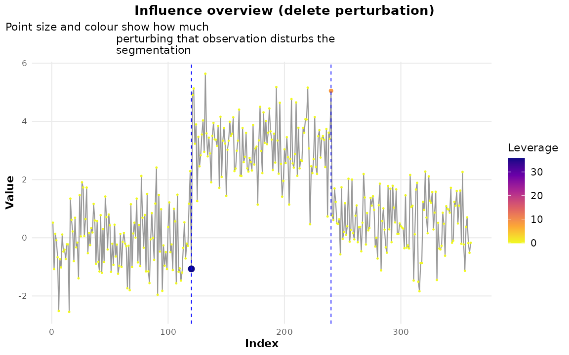

autoplot(inf, plot_type = "map")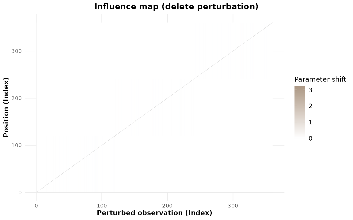

cpt_leverage() ranks the observations:

head(cpt_leverage(inf), 5)
#> # A tibble: 5 × 5
#>   index delta_n_cp max_shift param_shift leverage
#>   <int>      <int>     <dbl>       <dbl>    <dbl>
#> 1   120          0         2      3.25    35.8   
#> 2   240          0         1      0.0160   8.43  
#> 3   222          0         0      0.0226  -0.0292
#> 4    90          0         0      0.0212  -0.0374
#> 5   132          0         0      0.0209  -0.0388

Which setting

sens <- cpt_sensitivity(x, method = "pelt",
                        over = list(penalty = c(2, 8, 20, 60)))
sens
#> ggcpt_sensitivity (method: pelt, 4 settings)
#>   Swept: penalty
#>   Changepoints found: 2 to 46
#> 
#> # A tibble: 4 × 2
#>   penalty  n_cp
#>     <dbl> <int>
#> 1       2    46
#> 2       8     2
#> 3      20     2
#> 4      60     2
autoplot(sens)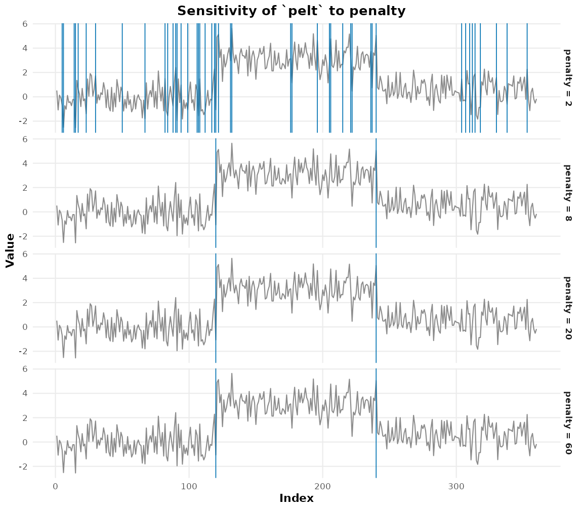

This is the direct answer to the commonest reviewer question about a changepoint analysis, and it is worth running before the analysis is written up rather than after it is questioned.

What the detector computed

Every detector evaluates something at every location and then keeps only the argmax. Three accessors give the discarded object back.

res_mosum <- cpt_detect(x, method = "mosum")
autoplot(res_mosum, type = "statistic")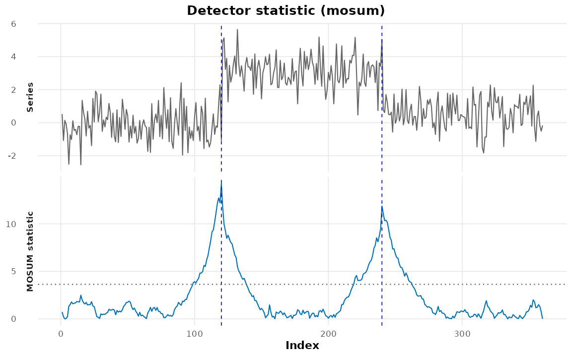

autoplot(type = "statistic") is a thin wrapper: ggcpt_statistic() is the plotting function itself, and cpt_statistic() returns the numbers behind it.

ggcpt_statistic(res_mosum)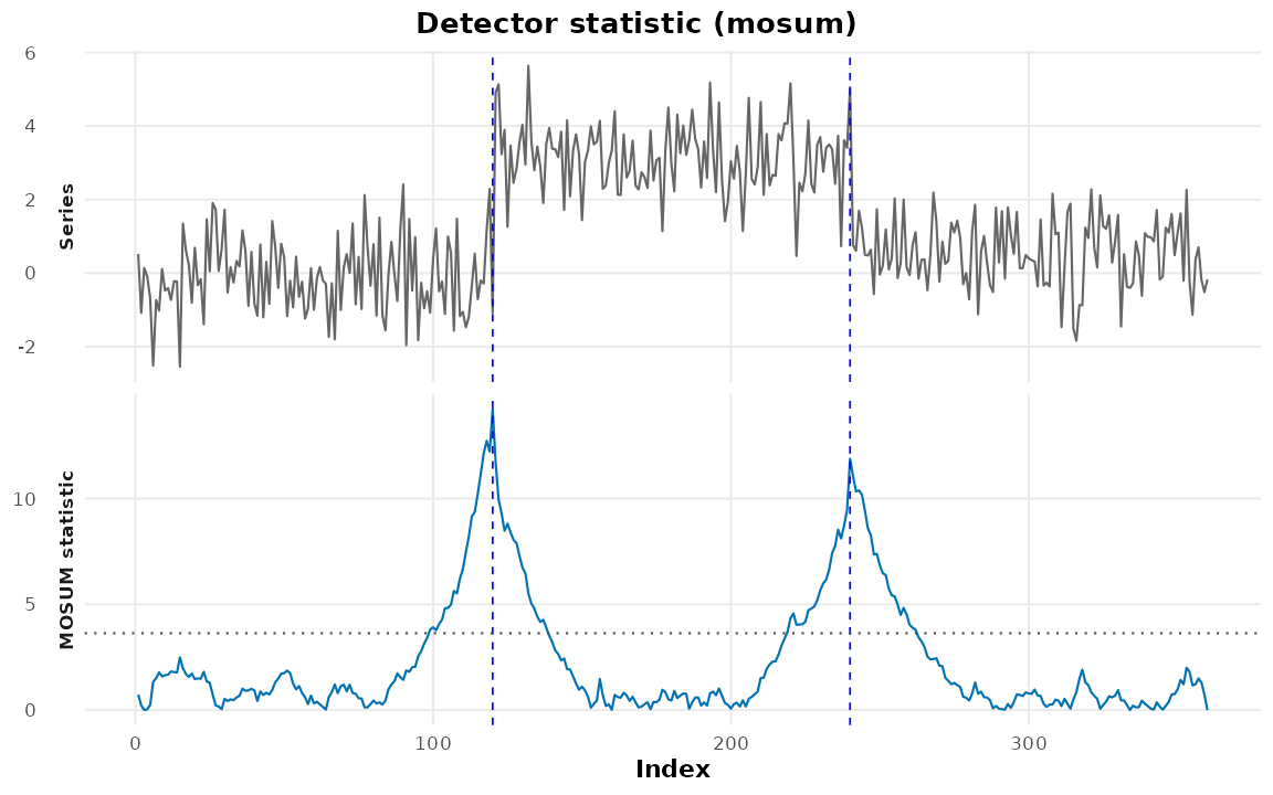

The scale-space view answers a question a single-bandwidth fit cannot: at which resolutions does this feature exist? A change visible only at a wide bandwidth is a slow shift; one visible only at a narrow bandwidth is a spike.

ggcpt_scale_space(res_mosum, bandwidths = c(15, 30, 60, 90))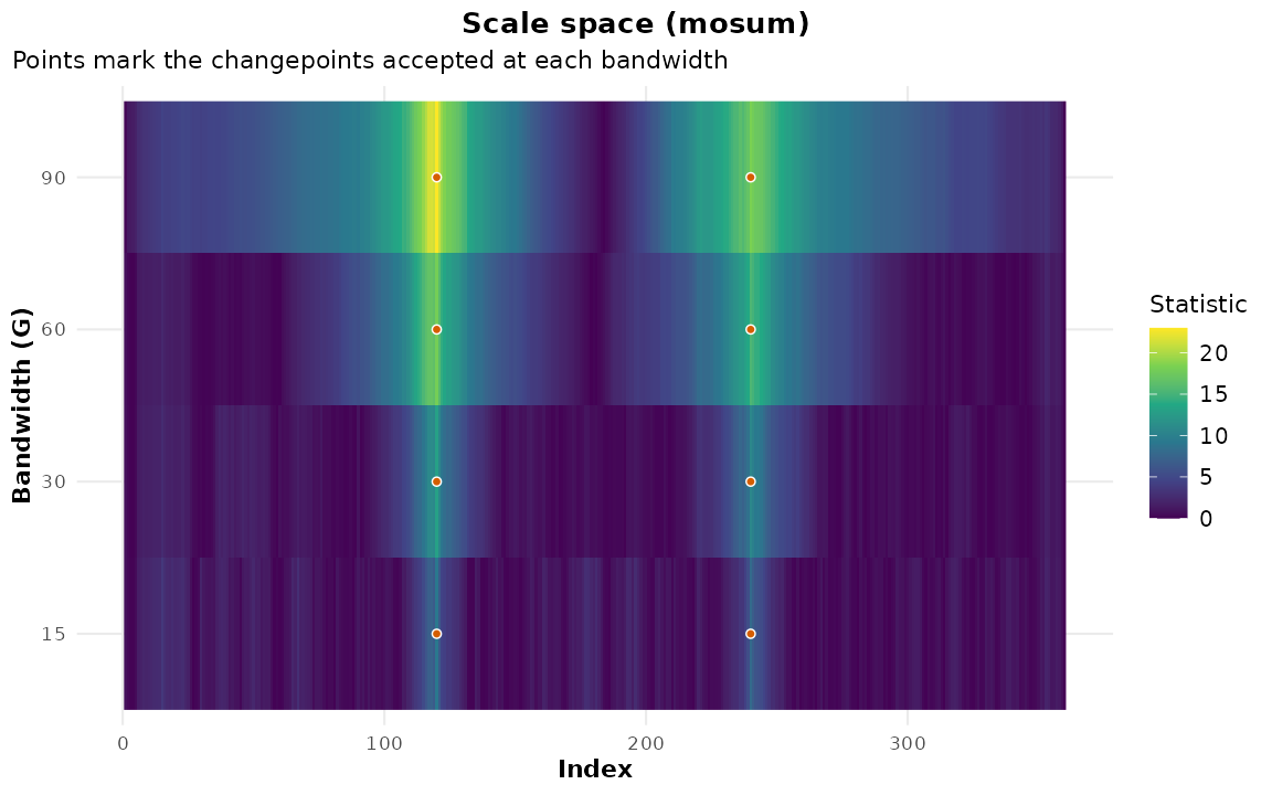

cpt_scale_space() returns the sweep as data, one row per (location, bandwidth) pair, so the picture can be counted rather than eyeballed. How many locations cross the threshold at each bandwidth:

ss <- cpt_scale_space(x, bandwidths = c(15, 30, 60, 90))
aggregate(significant ~ bandwidth, data = ss, FUN = sum)
#>   bandwidth significant
#> 1        15          20
#> 2        30          61
#> 3        60         171
#> 4        90         302

A wide bandwidth flags a broad neighbourhood of each change and a narrow one flags a few points, which is the resolution trade-off made numeric.

And the solution path shows the order in which candidates entered the model, and how decisively each beat the next:

ggcpt_solution_path(cpt_detect(x, method = "wbs"), max_steps = 20)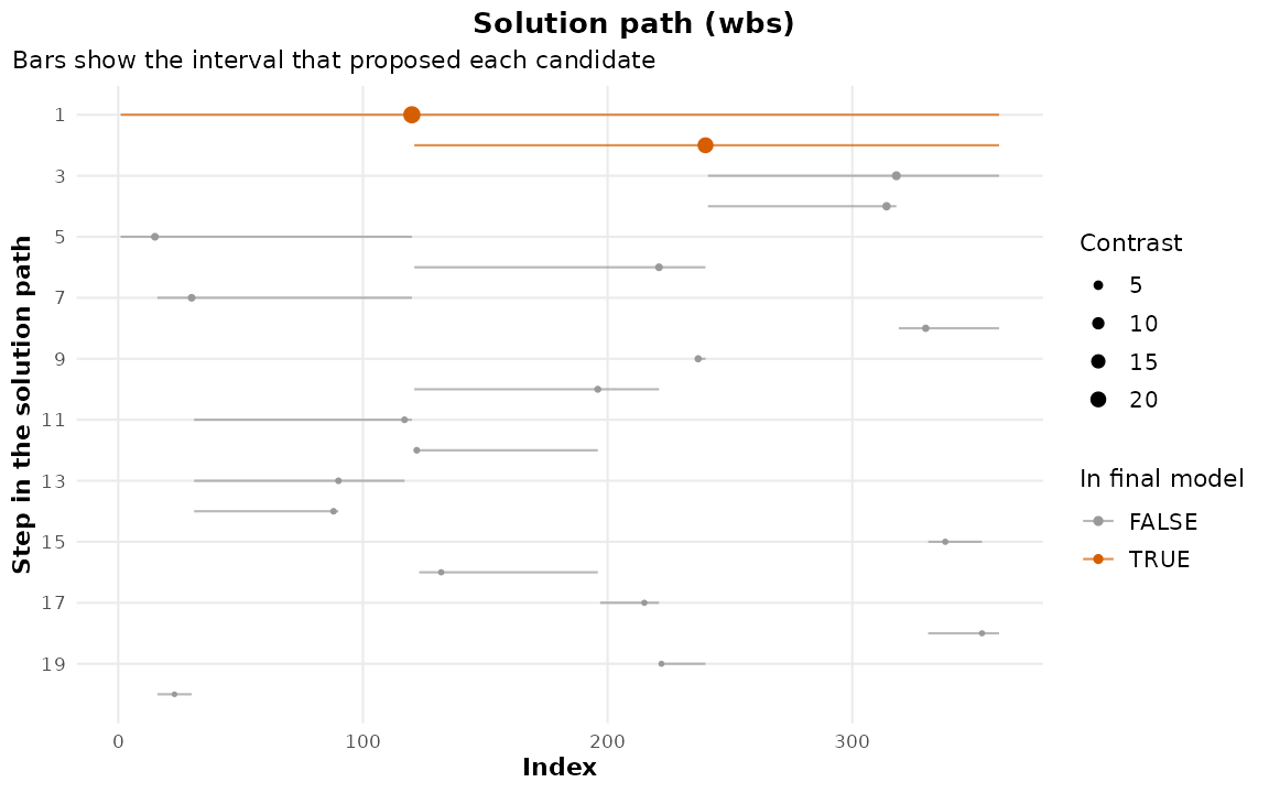

cpt_solution_path() is the same object as a tibble. The contrast column is the margin by which each candidate beat the next, and selected marks the ones the penalty kept — so the gap between the last selected row and the first rejected one is how close the decision was:

head(cpt_solution_path(cpt_detect(x, method = "wbs")), 5)
#> # A tibble: 5 × 6
#>    step    cp contrast start   end selected
#>   <int> <int>    <dbl> <int> <int> <lgl>   
#> 1     1   120    25.0      1   360 TRUE    
#> 2     2   240    20.2    121   360 TRUE    
#> 3     3   318     4.01   241   360 FALSE   
#> 4     4   314     3.65   241   318 FALSE   
#> 5     5    15     3.35     1   120 FALSE

An engine that exposes none of these says so, and names the ones that do:

cpt_statistic(fit)
#> Error:
#> ! Engine `pelt` does not expose a per-location statistic. These do: amoc, wbs, not, mosum, bcp, beast, nsp, pettitt, buishand, snht.

Putting it together

cat(head(cpt_report(fit, session = FALSE), 20), sep = "\n")

#> # Changepoint analysis report
#> 
#> - Method: `pelt`
#> - Change in: mean
#> - Penalty: MBIC
#> - Series length: 360
#> - Changepoints found: 2
#> - Detection runtime: 0.019 s
#> 
#> ## Changepoints
#> 
#> ```
#> # A tibble: 2 × 2
#>      cp cp_value
#>   <int>    <dbl>
#> 1   120    -1.07
#> 2   240     5.05
#> ```
#> 
#> ## Segments

References

Fryzlewicz, Piotr. 2024. “Narrowest Significance Pursuit: Inference for Multiple Change-Points in Linear Models.” Journal of the American Statistical Association 119 (546): 1633–46. https://doi.org/10.1080/01621459.2023.2211733.

Wilms, Ines, Rebecca Killick, and David S Matteson. 2022. “Graphical Influence Diagnostics for Changepoint Models.” Journal of Computational and Graphical Statistics 31 (3): 753–65. https://doi.org/10.1080/10618600.2021.2000873.

Zhang, Nancy R, and David O Siegmund. 2007. “A Modified Bayes Information Criterion with Applications to the Analysis of Comparative Genomic Hybridization Data.” Biometrics 63 (1): 22–32. https://doi.org/10.1111/j.1541-0420.2006.00662.x.

Zou, Changliang, Guanghui Wang, and Runze Li. 2020. “Consistent Selection of the Number of Change-Points via Sample-Splitting.” The Annals of Statistics 48 (1): 413–39. https://doi.org/10.1214/19-AOS1814.