Streaming and Online Monitoring

Every other vignette in this package segments a series that is already complete. This one does not. A monitor consumes observations as they arrive, and the question it answers is not where was the change but how long did you take to notice, and how often do you cry wolf. Those are different quantities, they are scored differently, and conflating them is the commonest mistake made with online detectors — including by retrospective plots that draw an alarm time as though it were a changepoint location.

So a monitor is a different object from a segmentation. Five functions:

Function	What it does
`cpt_monitor()`	build a stateful detector from a clean baseline
`cpt_update()`	push new observations through it
`alarms()`	the alarm log: when it fired, and on what statistic
`cpt_delay()`	score it — detection delay and false alarms
`cpt_replay()`	run a whole series through in one call

1. A monitor, one batch at a time

Start from a baseline the detector may assume is in control. edetector and ocd estimate their reference mean and scale from it; cpm derives its own from a start-up period and so does not need one.

set.seed(2026)
baseline <- rnorm(200)
mon <- cpt_monitor("edetector", baseline = baseline, alpha = 0.002)
mon
#> ggcpt_monitor (edetector -- native implementation)
#>   Baseline observations: 200
#>   Monitored observations: 0
#>   Alarms: 0
#>   Restart after alarm: TRUE (re-learning 20 observations)

Nothing has been monitored yet. Now feed it 120 observations from the same distribution — the in-control case, where the right answer is silence:

mon <- cpt_update(mon, rnorm(120))
mon
#> ggcpt_monitor (edetector -- native implementation)
#>   Baseline observations: 200
#>   Monitored observations: 120
#>   Alarms: 0
#>   Restart after alarm: TRUE (re-learning 20 observations)

Then a change arrives. The mean shifts by two standard deviations at observation 121 of the monitored stream, and the monitor sees it only one observation at a time:

mon <- cpt_update(mon, rnorm(80, mean = 2))
alarms(mon)
#> # A tibble: 2 × 3
#>    time statistic threshold
#>   <int>     <dbl>     <dbl>
#> 1   122      932.       500
#> 2   164      517.       500

The idiom is mon <- cpt_update(mon, new_obs): the monitor is returned because it is stateful, and each call appends to the same alarm log. The time column counts observations fed to the monitor, so the baseline is not on the clock.

2. Scoring: delay, not location

cpt_delay() matches each alarm to the change it plausibly detected, and counts the rest as false alarms.

d <- cpt_delay(mon, truth = 121)
d
#> ggcpt_delay
#>   True changes:      1
#>   Detected:          1
#>   Mean delay:        1
#>   Median delay:      1
#>   False alarms:      1
#>   Average run length: 200
#> 
#> # A tibble: 1 × 4
#>   truth alarm delay detected
#>   <int> <int> <dbl> <lgl>   
#> 1   121   122     1 TRUE

Read the three numbers that matter. Delay is how many observations passed between the change and the first alarm after it. False alarms are the alarms with no change behind them. Average run length is observations per false alarm — the in-control cost of running the monitor, and the quantity the thresholds are calibrated against.

Note what happened to the second alarm. Only the first alarm after a change counts as the detection, so the later one is charged as a false alarm even though the shift causing it is real. That is the right accounting for a monitor whose job is to raise one flag per change, and it is also a hint about relearn, which section 6 returns to.

tidy() and glance() give the same content as data:

glance(d)
#> # A tibble: 1 × 7
#>   n_changes n_detected mean_delay median_delay n_false_alarms   arl n_obs
#>       <int>      <int>      <dbl>        <dbl>          <int> <dbl> <int>
#> 1         1          1          1            1              1   200   200

cpt_metrics() is the wrong tool here. It asks whether the location was recovered, which a sequential procedure never claims: an alarm is deliberately late, so scoring it as a location estimate marks a correct detection wrong by exactly the delay.

autoplot(mon)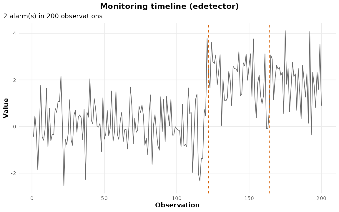

Monitored series with dashed vertical lines at each alarm

autoplot(d)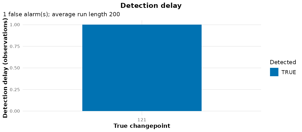

Bar chart of the detection delay at the true changepoint

3. Replaying a finished series

cpt_replay() does the update loop for you: it takes the leading observations as the baseline, streams the rest, and returns the same monitor object. This is how to study an online method’s alarm timeline retrospectively without pretending its alarms are changepoints.

stream <- c(rnorm(200), rnorm(200, mean = 2))
rep_e <- cpt_replay(stream, method = "edetector")
alarms(rep_e)
#> # A tibble: 3 × 3
#>    time statistic threshold
#>   <int>     <dbl>     <dbl>
#> 1   104      217.       100
#> 2   218      135.       100
#> 3   291      130.       100

The baseline offset is applied automatically, so truth is on the original clock of stream:

glance(cpt_delay(rep_e, truth = 200))
#> # A tibble: 1 × 7
#>   n_changes n_detected mean_delay median_delay n_false_alarms   arl n_obs
#>       <int>      <int>      <dbl>        <dbl>          <int> <dbl> <int>
#> 1         1          1          4            4              2   200   400

4. The three methods

`edetector` — the default, governed by `alpha`

A mixture Shiryaev–Roberts e-detector for a sub-Gaussian shift (Shin et al. 2023). For each candidate shift the increment is a likelihood ratio with unit mean under the null; the running statistics are combined by averaging, which keeps $M_t - t$ a mean-zero martingale, so optional stopping gives $E_\infty[\tau] \ge 1/\alpha$ — a finite-sample lower bound on the in-control average run length, with no calibration run. It is the one detector in this package implemented here rather than wrapped, because no R package implements e-detectors; print() labels it as such.

deltas is the set of shift sizes mixed over, in baseline standard deviations, each taken in both directions. The mixture is a uniform average, so adding a shift costs power at the ones already there rather than inflating the false-alarm rate — and betting on the wrong one is expensive. Eight replicates, median delay:

set.seed(2026)
delay_at <- function(deltas, shift, reps = 8, n = 200) {
  v <- vapply(seq_len(reps), function(i) {
    s <- c(rnorm(n), rnorm(n, mean = shift))
    cpt_delay(cpt_replay(s, method = "edetector", deltas = deltas),
              truth = n)$median_delay
  }, numeric(1))
  median(v, na.rm = TRUE)
}
data.frame(
  shift = c(0.75, 3),
  mixture_0.5_1_2 = c(delay_at(c(0.5, 1, 2), 0.75), delay_at(c(0.5, 1, 2), 3)),
  only_0.5 = c(delay_at(0.5, 0.75), delay_at(0.5, 3)),
  only_3 = c(delay_at(3, 0.75), delay_at(3, 3))
)
#>   shift mixture_0.5_1_2 only_0.5 only_3
#> 1  0.75            14.5     11.0     37
#> 2  3.00             2.0      4.5      2

A detector that mixes only over a 3-sigma shift takes several times as long to notice a 0.75-sigma one, while the mixture is close to the best single choice at both sizes. That is the argument for mixing: it buys robustness to not knowing the change size, at a small cost when you do.

`cpm` — governed by `arl0`

cpm’s sequential change-point model (Ross 2015), with a distribution-free statistic (cpm_type, "Mann-Whitney" by default) and a threshold calibrated to a target in-control average run length.

mon_cpm <- cpt_monitor("cpm", arl0 = 500)
mon_cpm <- cpt_update(mon_cpm, rnorm(120))
mon_cpm <- cpt_update(mon_cpm, rnorm(80, mean = 2))
alarms(mon_cpm)
#> # A tibble: 1 × 3
#>    time statistic threshold
#>   <int>     <dbl>     <dbl>
#> 1   125         0        NA
glance(cpt_delay(mon_cpm, truth = 121))
#> # A tibble: 1 × 7
#>   n_changes n_detected mean_delay median_delay n_false_alarms   arl n_obs
#>       <int>      <int>      <dbl>        <dbl>          <int> <dbl> <int>
#> 1         1          1          4            4              0   Inf   200

cpm does the threshold comparison inside the engine, so threshold is NA in its alarm log rather than an invented number, and the statistic column is not informative for it either. The alarm time is the whole signal from cpm; the statistic trace is what edetector and ocd provide and cpm does not.

`alpha` and `arl0` are alternative parameterisations, not two knobs

cpt_monitor() exposes both because the two engines are calibrated in different currencies, and each ignores the other’s. edetector honours alpha (its threshold is $1/\alpha$ ); cpm honours arl0. Setting arl0 on an e-detector, or alpha on cpm, changes nothing.

ic <- rnorm(400)
vapply(c(0.05, 0.01, 0.001),
       function(a) nrow(alarms(cpt_replay(ic, method = "edetector",
                                          alpha = a))),
       numeric(1))
#> [1] 7 3 0
nrow(alarms(cpt_replay(ic, method = "edetector", arl0 = 5000)))
#> Warning: `arl0` does not affect `method = "edetector"`, which is tuned by
#> `alpha`, `deltas`. See ?cpt_monitor.
#> [1] 3

Three alphas, three false-alarm counts; then arl0 = 5000 on the same stream, which reproduces the default-alpha result exactly because the argument is not read – and cpt_monitor() says so, because an argument that is accepted and then ignored is worth a warning rather than an unchanged answer. The rough translation is $\mathrm{ARL}_0 \approx 1/\alpha$ , so alpha = 0.002 and arl0 = 500 ask for comparable strictness.

`ocd` — multivariate only

ocd’s high-dimensional multiscale detector (Chen et al. 2022) tracks a projection of the whole vector, and requires at least two coordinates. On a single series it does not fall back to a univariate statistic; it stops, and says which methods do read one series:

cpt_monitor("ocd", baseline = rnorm(100))
#> Error:
#> ! Method `ocd` is high-dimensional and needs at least two coordinates, but `baseline` has 1. Use method = "edetector" or "cpm" for one series.

Given a matrix with rows as time points it monitors all coordinates jointly, and the alarms are shared across them:

set.seed(11)
base_mv <- matrix(rnorm(200 * 3), ncol = 3)
mon_ocd <- cpt_monitor("ocd", baseline = base_mv, patience = 200,
                       mc_reps = 30)
stream_mv <- rbind(matrix(rnorm(60 * 3), ncol = 3),
                   matrix(rnorm(60 * 3, mean = 1.2), ncol = 3))
mon_ocd <- cpt_update(mon_ocd, stream_mv)
glance(cpt_delay(mon_ocd, truth = 61))
#> # A tibble: 1 × 7
#>   n_changes n_detected mean_delay median_delay n_false_alarms   arl n_obs
#>       <int>      <int>      <dbl>        <dbl>          <int> <dbl> <int>
#> 1         1          1          5            5              0   Inf   120

Two practical notes. The statistic reported is ocd’s normalised statistic, already divided by its own threshold, so the comparison point is 1 — printing the raw thresholds alongside it would show an alarm at 1.10 against a threshold of 16.4 and read as a bug. And the Monte Carlo threshold calibration is the expensive part of building the monitor: a minute or more at the default patience = 5000, which is why mc_reps is lowered here. Pass thresh directly when you already have thresholds.

5. Delay is a function of shift size

The whole point of an online detector is that a bigger change is noticed sooner. This is small enough to measure directly — ten replicates per cell, median over replicates:

set.seed(2026)
median_delay <- function(shift, method, reps = 10, n = 200) {
  d <- vapply(seq_len(reps), function(i) {
    s <- c(rnorm(n), rnorm(n, mean = shift))
    cpt_delay(cpt_replay(s, method = method), truth = n)$median_delay
  }, numeric(1))
  median(d, na.rm = TRUE)
}
grid <- expand.grid(shift = c(1, 2, 3),
                    method = if (has_cpm) c("edetector", "cpm") else "edetector",
                    stringsAsFactors = FALSE)
grid$median_delay <- mapply(median_delay, grid$shift, grid$method)
grid
#>   shift    method median_delay
#> 1     1 edetector          7.0
#> 2     2 edetector          4.0
#> 3     3 edetector          1.5
#> 4     1       cpm          9.0
#> 5     2       cpm          4.5
#> 6     3       cpm          4.0

Ten replicates is a noisy estimate of a median, and the table above will wobble with the seed. A larger run of the same design gives median detection delays of roughly 12, 4 and 2 observations for edetector at shifts of 1, 2 and 3 standard deviations, and 11, 5 and 4 for cpm. Two things are worth taking from that. Delay falls steeply in the shift size, so a monitor tuned on a large change will feel unusably slow on a small one. And the ordering of the two detectors is not fixed: at 1 sigma they are within an observation or two of each other, and the small run above and the larger one disagree about which is ahead, while edetector is clearly quicker once the change is obvious.

6. Assumptions: the thresholds are for independent observations

Both calibrations — the e-detector’s $1/\alpha$ bound and cpm’s arl0 — assume the in-control observations are independent. Under the null on iid noise they hold up. Measured on 2000-observation in-control streams at the defaults, cpm raises about 3.7 false alarms against the 4 that arl0 = 500 implies by construction, and edetector about 13.

Serial dependence breaks both, and not gently. Autocorrelated noise wanders; a detector that reads a wander as a level shift alarms on it.

set.seed(3)
false_alarms <- function(method, gen, reps = 5, n = 400) {
  mean(vapply(seq_len(reps),
              function(i) nrow(alarms(cpt_replay(gen(n), method = method))),
              numeric(1)))
}
iid <- function(n) rnorm(n)
ar1 <- function(n) as.numeric(stats::arima.sim(list(ar = 0.7), n))
methods <- if (has_cpm) c("edetector", "cpm") else "edetector"
data.frame(
  method = methods,
  iid = vapply(methods, false_alarms, numeric(1), gen = iid),
  ar1_rho_0.7 = vapply(methods, false_alarms, numeric(1), gen = ar1),
  row.names = NULL
)
#>      method iid ar1_rho_0.7
#> 1 edetector 1.8         7.4
#> 2       cpm 0.6         6.2

Both inflate badly at $\rho = 0.7$ , cpm by roughly tenfold in a larger run of the same comparison. Neither is broken — they are answering the question they were calibrated for — but a nominal arl0 = 500 on autocorrelated data is not a 500-observation run length, and reporting it as one overstates the evidence behind every alarm. The options, in order of how much they ask of you:

Pre-whiten. Fit an AR model to the baseline and monitor the residuals. Cheap, and it restores the calibration when the model is about right.
Aggregate. Monitor block means rather than raw observations. The dependence between blocks is weaker; the cost is delay measured in blocks.
Recalibrate empirically. Simulate in-control streams with the dependence you actually have, and set alpha or arl0 to the level that delivers the run length you want. This is the honest route when the noise model is not AR.

Two further assumptions, worth stating because they are easy to miss. The baseline must be clean: edetector and ocd take their reference mean and scale from it, so a change inside the baseline is inherited as the in-control state and the real change afterwards may be invisible. And relearn (20 observations by default) is not cosmetic. A real change is persistent, so a monitor that restarts against the stale pre-change baseline alarms again on the very next observation and keeps alarming for the rest of the stream — reporting one change as hundreds, all but the first of which cpt_delay() counts as false alarms. Set relearn = 0 only when you want to see every threshold crossing.

nrow(alarms(cpt_replay(stream, method = "edetector", relearn = 20)))
#> [1] 3
nrow(alarms(cpt_replay(stream, method = "edetector", relearn = 0)))
#> [1] 36

7. What to report

For an online analysis, the summary that belongs in a paper is glance(cpt_delay(...)): how many changes there were, how many were detected, the delay distribution, the false-alarm count and the realised run length. A list of alarm times without the delay accounting is not an evaluation, and a covering or F1 score computed against alarm times is a category error. Delay against false alarms has been the currency of sequential monitoring since Page (1954); the tooling here just makes the accounting automatic.

glance(cpt_delay(rep_e, truth = 200))
#> # A tibble: 1 × 7
#>   n_changes n_detected mean_delay median_delay n_false_alarms   arl n_obs
#>       <int>      <int>      <dbl>        <dbl>          <int> <dbl> <int>
#> 1         1          1          4            4              2   200   400

References

Chen, Yudong, Tengyao Wang, and Richard J Samworth. 2022. “High-Dimensional, Multiscale Online Changepoint Detection.” Journal of the Royal Statistical Society: Series B 84 (1): 234–66.

Page, Ewan S. 1954. “Continuous Inspection Schemes.” Biometrika 41 (1/2): 100–115.

Ross, Gordon J. 2015. “Parametric and Nonparametric Sequential Change Detection in r: The Cpm Package.” Journal of Statistical Software 66 (3): 1–20.

Shin, Jaehyeok, Aaditya Ramdas, and Alessandro Rinaldo. 2023. “E-Detectors: A Nonparametric Framework for Sequential Change Detection.” The New England Journal of Statistics in Data Science 1 (2): 229–60. https://doi.org/10.51387/23-NEJSDS49.

Youzhi YuUniversity of Chicago