Control Charts Are Changepoint Detectors

Youzhi Yu
University of Chicago

Statistical process control and sequential changepoint detection are the same mathematics in two vocabularies. A CUSUM chart is a sequential likelihood-ratio test for a shift in the mean; an EWMA chart is its smoothed relative; the in-control average run length a quality engineer calls ARL0 is the false-alarm budget a changepoint paper calls ARL0 too. This page translates between the two, with the charts cpt_monitor() runs.

The dictionary

Process control	Changepoint detection	In this package
Phase I: establish the in-control process	Offline detection on the history	cpt_detect(history)
Phase II: monitor new data	Sequential detection	cpt_monitor() and cpt_update()
Out-of-control signal	Alarm	alarms(monitor)
In-control ARL (ARL0)	Average run length to a false alarm	arl0 =
Out-of-control ARL (ARL1)	Detection delay	cpt_delay()
CUSUM reference value k	Half the shift tuned for	k = 0.5 for a one-sigma shift
Decision interval h, EWMA limit L	Threshold	solved from arl0, or limit =

Phase I: is the history in control?

A chart is only as good as the baseline it standardises by. Check the history for changes before trusting it:

set.seed(2030)
history <- rnorm(400, mean = 10, sd = 2)
cpt_detect(history, method = "pelt", change_in = "meanvar")$changepoints
#> # A tibble: 0 × 2
#> # ℹ 2 variables: cp <int>, cp_value <dbl>

No changepoints: the history can serve as the baseline.

Phase II: monitor

stream <- c(rnorm(200, 10, 2), rnorm(150, 12, 2))
cusum <- cpt_update(cpt_monitor("cusum", baseline = history, arl0 = 500),
                    stream)
ewma <- cpt_update(cpt_monitor("ewma", baseline = history, arl0 = 500),
                   stream)
cusum
#> ggcpt_monitor (cusum, native implementation)
#>   Chart: k = 0.5, h = 5.071 (in-control ARL 500)
#>   Baseline observations: 400
#>   Monitored observations: 350
#>   Alarms: 1
#>   Restart after alarm: TRUE (re-learning 20 observations)
#> 
#> # A tibble: 1 × 3
#>    time statistic threshold
#>   <int>     <dbl>     <dbl>
#> 1   206      5.55      5.07

autoplot(cusum, plot_type = "control_chart")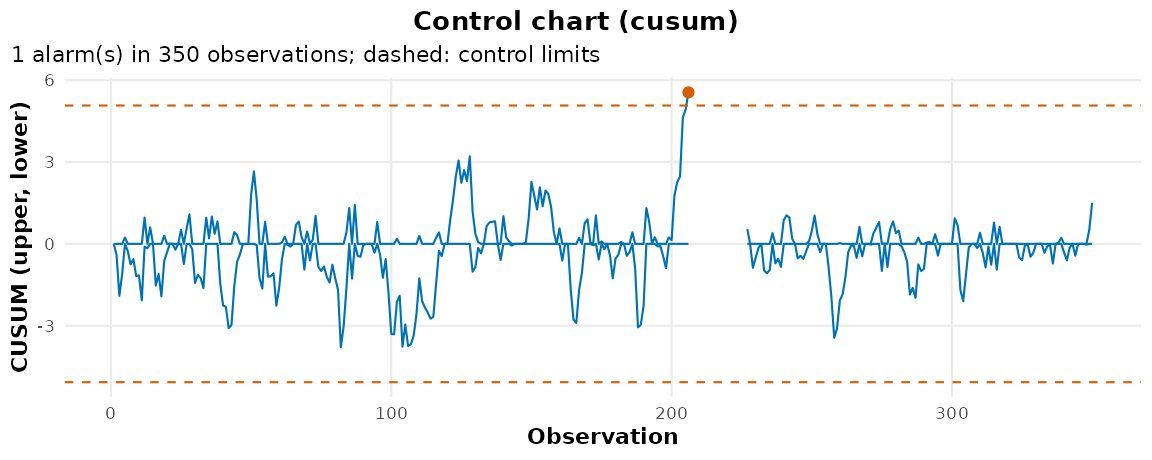

autoplot(ewma, plot_type = "control_chart")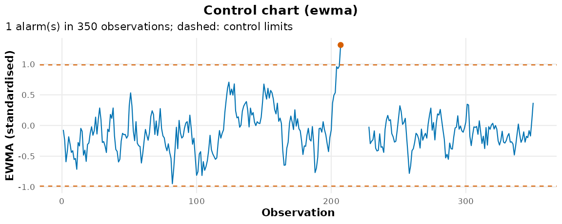

The shift of one standard deviation arrives at observation 201. Scored the way the sequential literature scores it, by delay and false alarms:

glance(cpt_delay(cusum, truth = 200))
#> # A tibble: 1 × 7
#>   n_changes n_detected mean_delay median_delay n_false_alarms   arl n_obs
#>       <int>      <int>      <dbl>        <dbl>          <int> <dbl> <int>
#> 1         1          1          6            6              0   Inf   350
glance(cpt_delay(ewma, truth = 200))
#> # A tibble: 1 × 7
#>   n_changes n_detected mean_delay median_delay n_false_alarms   arl n_obs
#>       <int>      <int>      <dbl>        <dbl>          <int> <dbl> <int>
#> 1         1          1          7            7              0   Inf   350

The calibration

Both limits are solved for arl0 by the Markov-chain approximation of the run length (Brook and Evans 1972 for the CUSUM; Lucas and Saccucci 1990 for the EWMA), which reproduces the published tables: a CUSUM with k = 0.5 runs 168 in control at h = 4 and 465 at h = 5. Through the monitor itself, against the target:

cal <- cpt_calibration
cal[grepl("cusum|ewma", cal$call), c("call", "nominal", "realised", "mcse")]
#> # A tibble: 2 × 4
#>   call                                 nominal realised  mcse
#>   <chr>                                  <dbl>    <dbl> <dbl>
#> 1 "cpt_monitor(\"cusum\", arl0 = 500)"     500      495    25
#> 2 "cpt_monitor(\"ewma\", arl0 = 500)"      500      531    28

The calibration treats the baseline’s mean and standard deviation as exact, so a longer baseline keeps the run length on target: a few hundred observations is a good minimum.

Choosing the chart

You expect	Use
A sustained shift of about one standard deviation	cpt_monitor("cusum", k = 0.5)
A small shift, half a standard deviation or less	cpt_monitor("ewma", lambda = 0.05)
A shift of unknown size	cpt_monitor("edetector"), which mixes over sizes with a run-length guarantee
A change in distribution, not just the mean	cpt_monitor("cpm")
Many streams at once	cpt_monitor("ocd")

Rational subgroups, Western Electric run rules and capability indices are part of formal process control and are not modelled here; for a quality programme built on them, use a dedicated package such as qcc, and use this one for the detection, the delay accounting and the plots.

References

Brook, D. and Evans, D. A. (1972). An approach to the probability distribution of CUSUM run length. Biometrika, 59(3), 539-549.

Lucas, J. M. and Saccucci, M. S. (1990). Exponentially weighted moving average control schemes: properties and enhancements. Technometrics, 32(1), 1-12.

Page, E. S. (1954). Continuous inspection schemes. Biometrika, 41(1/2), 100-115.

Roberts, S. W. (1959). Control chart tests based on geometric moving averages. Technometrics, 1(3), 239-250.