Beyond the Location: Which, How Sure, and What If

Youzhi Yu
University of Chicago

A detector answers where. Every applied field then asks the same few questions: which of the measured quantities changed, how sure the location is, what the series would have done otherwise, whether the change was a jump at all, and, with many series, which ones changed. This page answers each with one function, on data where the answer is known.

Which coordinates changed

Testing each sensor at the detected changepoint is the obvious answer and an invalid one: the location was chosen where the evidence across all of them peaks, so an unchanged sensor is tested at the split most favourable to it. cpt_attribute() scores each coordinate by the maximum of a rank statistic over every split instead (ARM, Peng et al. 2026), so the certificate cannot depend on how the location was found.

set.seed(1)
n <- 200
X <- matrix(rnorm(n * 8), n, 8, dimnames = list(NULL, paste0("sensor", 1:8)))
X[101:n, 3] <- X[101:n, 3] + 1.2      # a shift in sensor3
X[101:n, 6] <- X[101:n, 6] * 2.5      # a scale change in sensor6
fit_mv <- cpt_detect(X, method = "ecp")
att <- cpt_attribute(fit_mv, B = 499, seed = 1)
att
#> ggcpt_attribution (ARM: attribution by rank maxima)
#>   Controls:           family-wise error (Westfall-Young) at 0.05
#>   Permutations:       499
#>   Changepoint 100:    2 of 8: sensor3 (location), sensor6 (scale)
#> 
#> # A tibble: 8 × 13
#>      cp coordinate statistic statistic_location statistic_scale p_value
#>   <int> <chr>          <dbl>              <dbl>           <dbl>   <dbl>
#> 1   100 sensor1         2.57               2.15           2.57    0.316
#> 2   100 sensor2         1.59               1.59           0.996   0.952
#> 3   100 sensor3         7.10               7.10           1.25    0.002
#> 4   100 sensor4         1.76               1.76           1.18    0.878
#> 5   100 sensor5         2.16               1.38           2.16    0.564
#> 6   100 sensor6         6.48               2.51           6.48    0.002
#> 7   100 sensor7         3.06               3.06           2.70    0.1  
#> 8   100 sensor8         2.06               2.06           1.88    0.704
#> # ℹ 7 more variables: p_adjusted <dbl>, changed <lgl>, type <chr>,
#> #   window_start <int>, window_end <int>, n_window <int>, source <chr>

autoplot(att)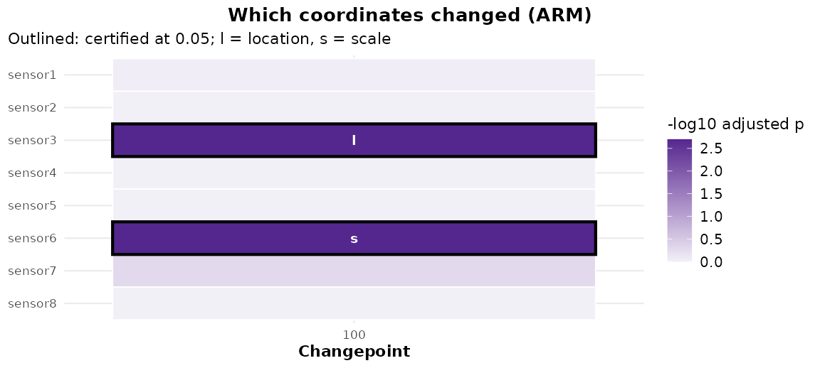

The two changed sensors are certified, each with its type, and the six that did not change are left alone. Measured on the calibration design, the family-wise error over the unchanged coordinates is:

cal <- cpt_calibration
cal[grepl("cpt_attribute", cal$call), c("setting", "nominal", "realised", "mcse")]
#> # A tibble: 1 × 4
#>   setting                                                nominal realised   mcse
#>   <chr>                                                    <dbl>    <dbl>  <dbl>
#> 1 ARM, Westfall-Young, B = 199; 8 t(3) coordinates, 2 s…    0.05    0.031 0.0055

How sure is the location, with no model

cpt_confint(method = "conformal") returns a set of locations that holds the true one with probability at least the level, for any distribution of the noise, provided the observations within each segment are exchangeable (Hore and Ramdas 2026). Here on heavy-tailed noise, where a Gaussian interval has no footing:

set.seed(2)
y <- c(rt(150, df = 3), rt(150, df = 3) + 1.5)
fit <- cpt_detect(y, method = "pelt")
ci <- cpt_confint(fit, method = "conformal", B = 199, seed = 1)
ci
#> # A tibble: 1 × 6
#>      cp ci_lower ci_upper level source    set_size
#>   <int>    <int>    <int> <dbl> <chr>        <int>
#> 1   149      137      151  0.95 conformal       13

prof <- attr(ci, "profile")
ggplot(prof, aes(position, p_value)) +
  geom_col(width = 1, fill = "#5e3c99") +
  geom_hline(yintercept = 0.05, linetype = "dashed") +
  coord_cartesian(xlim = c(120, 180)) +
  labs(x = "Candidate location", y = "Conformal p-value")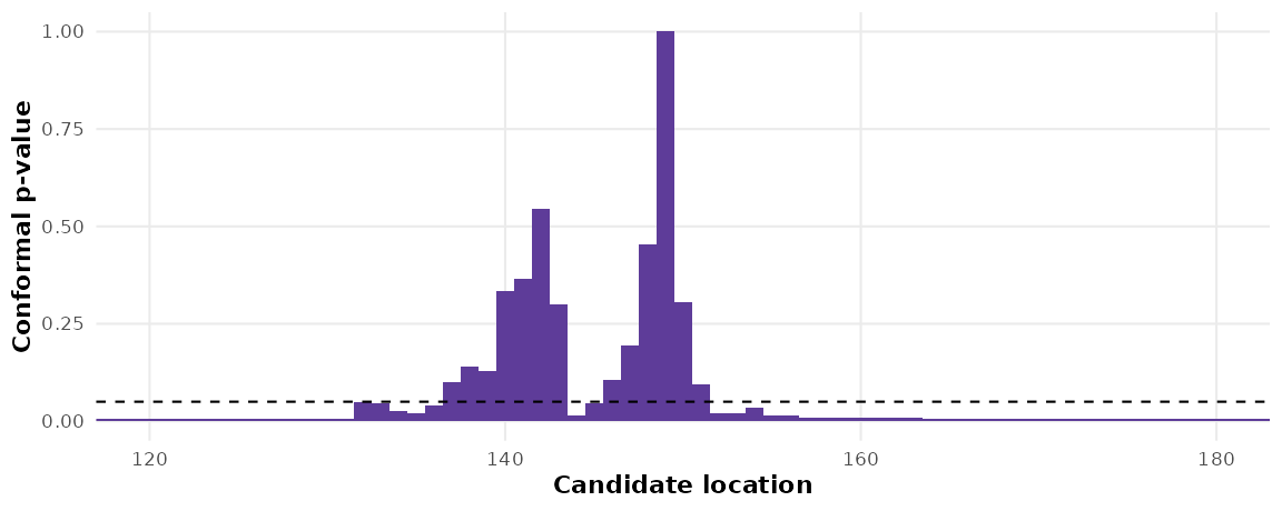

The coverage, measured on the calibration design and against the bootstrap:

cal[grepl("location", cal$guarantee) & grepl("conformal|bootstrap", cal$call),
    c("call", "nominal", "realised", "mcse")]
#> # A tibble: 2 × 4
#>   call                                                 nominal realised   mcse
#>   <chr>                                                  <dbl>    <dbl>  <dbl>
#> 1 "cpt_confint(cpt_detect(x), method = \"bootstrap\")"    0.95    0.968 0.0056
#> 2 "cpt_confint(cpt_detect(x), method = \"conformal\")"    0.95    0.97  0.0054

cpt_confint_coverage() runs the same study for your own length, jump and noise.

What would have happened

cpt_counterfactual() carries the segment before each change forward with its own model, with a prediction band, and the gap is the effect in the data’s units: the figure interrupted-time-series studies report.

nile <- cpt_detect(Nile, method = "amoc", change_in = "meanvar")
cf <- cpt_counterfactual(nile)
glance(cf)
#> # A tibble: 1 × 5
#>      cp     n mean_effect cumulative_effect share_outside
#>   <int> <int>       <dbl>             <dbl>         <dbl>
#> 1    28    72       -248.           -17840.         0.389
autoplot(cf)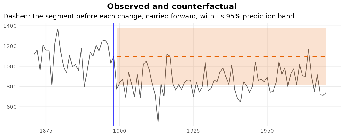

Was it a jump?

Every engine looks for a jump, and given a transition that took thirty observations it reports one confidently placed changepoint in the middle. cpt_abruptness() fits a step and a ramp at each changepoint and reports the transition width with an interval:

sim <- cpt_simulate(300, changepoints = 150, params = c(0, 3),
                    transition = 40, seed = 3)
ab <- cpt_abruptness(cpt_detect(sim$value, method = "pelt"))
ab
#> ggcpt_abruptness (a step against a ramp at each changepoint)
#>   Changepoint 148:    gradual, transition width 24 (8 to 31)
#> 
#> # A tibble: 1 × 10
#>      cp window_start window_end width width_lower width_upper centre statistic
#>   <int>        <int>      <int> <dbl>       <dbl>       <dbl>  <dbl>     <dbl>
#> 1   148            1        300    24           8          31   150.      5.62
#> # ℹ 2 more variables: p_value <dbl>, verdict <chr>
autoplot(ab)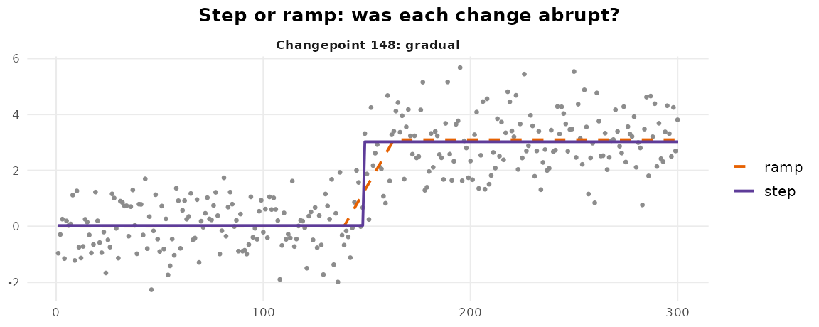

A change that comes back

An outbreak that subsides or a fault that is repaired is a stretch away from a baseline, not a new regime. CAPA models exactly that, and reports the stretches and the single outliers:

set.seed(4)
z <- c(rnorm(150), rnorm(40, 2.5), rnorm(150))
z[60] <- 7
ep <- cpt_detect(z, method = "capa")
cpt_regions(ep)
#> # A tibble: 2 × 7
#>   start   end length type       coordinates mean_change strength
#>   <int> <int>  <int> <chr>      <chr>             <dbl>    <dbl>
#> 1    60    60      1 point      V1                NA        5.93
#> 2   151   190     40 collective V1                 3.75    NA
autoplot(ep)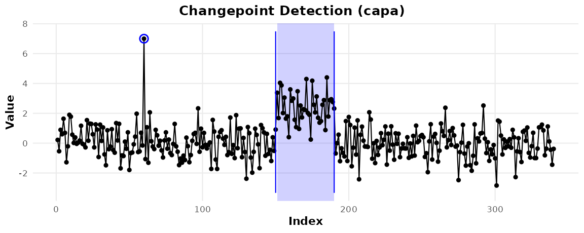

How many changes, and which series

cpt_k_weights() turns the criterion curve of cpt_select() into weights over the number of changes, and averages the candidate segmentations into a probability at each location:

set.seed(5)
w <- cpt_k_weights(cpt_select(c(rnorm(100), rnorm(100, 0.8), rnorm(100)),
                              criterion = "bic", k_max = 6))
w
#> ggcpt_k_weights (weights over the number of changepoints, from bic)
#>   Chosen:             K = 2, weight 0.596
#>   Largest weights:    K = 2: 0.596; K = 3: 0.370; K = 4: 0.032
#>   95% of the weight:  K in {2, 3}
#> 
#> # A tibble: 7 × 5
#>       k value  delta     weight chosen
#>   <int> <dbl>  <dbl>      <dbl> <lgl> 
#> 1     0  35.1 23.0   0.00000605 FALSE 
#> 2     1  30.7 18.6   0.0000539  FALSE 
#> 3     2  12.1  0     0.596      TRUE  
#> 4     3  13.1  0.952 0.370      FALSE 
#> 5     4  17.9  5.82  0.0325     FALSE 
#> 6     5  25.4 13.3   0.000777   FALSE 
#> 7     6  33.7 21.6   0.0000124  FALSE
autoplot(w)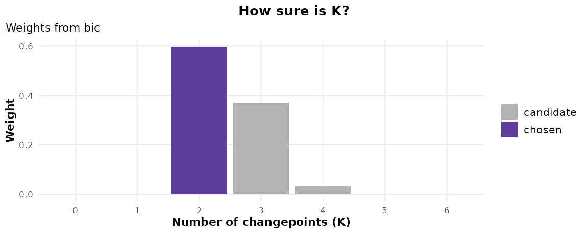

And for a panel, cpt_screen() tests every series for a change anywhere and controls the false discovery rate across them:

set.seed(6)
panel <- c(lapply(1:52, function(i) rnorm(120)),
           lapply(1:8, function(i) c(rnorm(60), rnorm(60, 1.2))))
names(panel) <- paste0("store", 1:60)
sc <- cpt_screen(panel)
glance(sc)
#> # A tibble: 1 × 5
#>   n_series n_flagged alpha control test   
#>      <int>     <int> <dbl> <chr>   <chr>  
#> 1       60         9  0.05 fdr     pettitt
autoplot(sc)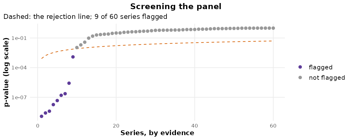

References

Fisch, A. T. M., Eckley, I. A. and Fearnhead, P. (2022). A linear time method for the detection of collective and point anomalies. Statistical Analysis and Data Mining, 15(4), 494-508.

Hore, R. and Ramdas, A. (2026). Conformal changepoint localization. arXiv:2602.06267.

Peng, C., Wu, M., Yan, Q., Chen, D. and Shen, Z. (2026). ARM: Detector-agnostic changepoint attribution with finite-sample error control. arXiv:2608.01691.