Supervised Changepoint Detection

Almost every changepoint method in this package is unsupervised: it picks a penalty by an information criterion and hopes the criterion matches what you would have said. Supervised changepoint detection (Hocking et al. 2013) does something different. An expert marks regions of the series as containing a change or not, accuracy is measured in label errors against those marks, and the penalty is learned from them.

Three things make it worth a vignette of its own:

it consistently beats unsupervised penalties on labelled data;
it gives a defensible answer to “what penalty should I use?” that does not depend on a modelling assumption;
its central object is a rectangle drawn over a time series, which is a ggplot2-native idea with no ggplot2-native implementation elsewhere.

Labels

A label is a stretch of the series with an assertion attached.

set.seed(2026)
x <- c(rnorm(80), rnorm(80, 4), rnorm(80, 1))

labs <- cpt_labels(
  start  = c(  1,  60, 100, 140, 190),
  end    = c( 55,  95, 135, 185, 240),
  change = c("no_change", "one_change", "no_change", "one_change",
             "no_change")
)
labs
#> # A tibble: 5 × 5
#>   label_id series start   end change    
#>      <int> <chr>  <int> <int> <chr>     
#> 1        1 NA         1    55 no_change 
#> 2        2 NA        60    95 one_change
#> 3        3 NA       100   135 no_change 
#> 4        4 NA       140   185 one_change
#> 5        5 NA       190   240 no_change

Three kinds, and the distinction matters:

"change" — at least one changepoint lies here.
"one_change" — exactly one does. Stricter, and the only one that makes a false positive inside a positive region detectable.
"no_change" — none does. Without these, a detector is never penalised for a false positive, and the learned penalty collapses to zero.

Because labels are just a tidy tibble, they draw directly:

d <- data.frame(t = seq_along(x), y = x)
ggplot(d, aes(t, y)) +
  geom_cpt_label(aes(xmin = start, xmax = end, fill = change), data = labs) +
  geom_line(colour = "grey30") +
  scale_fill_cpt_label() +
  labs(fill = "Label", x = "Index", y = "Value")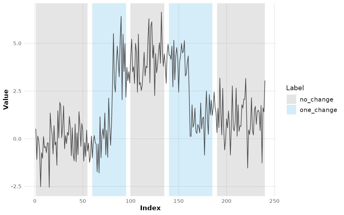

Series with shaded label regions behind it, coloured by what each label asserts

If you already have a plain ground-truth changepoint set — the kind cpt_metrics() takes — as_cpt_labels() converts it, positives and negatives together, so the package has one notion of an annotation rather than two:

as_cpt_labels(c(80, 160), n = 240, margin = 5)
#> # A tibble: 5 × 5
#>   label_id series start   end change    
#>      <int> <chr>  <int> <int> <chr>     
#> 1        3 NA         1    74 no_change 
#> 2        1 NA        75    85 one_change
#> 3        4 NA        86   154 no_change 
#> 4        2 NA       155   165 one_change
#> 5        5 NA       166   239 no_change

Scoring a segmentation

fit <- cpt_detect(x, method = "pelt")
err <- cpt_label_error(fit, labs)
err
#> cpt_label_error (5 label(s))
#>   correct: 5   false positives: 0   false negatives: 0
#>   total label errors: 0
#> 
#> # A tibble: 5 × 7
#>   label_id series start   end change     n_changes status 
#>      <int> <chr>  <int> <int> <chr>          <int> <chr>  
#> 1        1 NA         1    55 no_change          0 correct
#> 2        2 NA        60    95 one_change         1 correct
#> 3        3 NA       100   135 no_change          0 correct
#> 4        4 NA       140   185 one_change         1 correct
#> 5        5 NA       190   240 no_change          0 correct

The three-colour status shading turns model evaluation into a picture:

ggplot(d, aes(t, y)) +
  geom_cpt_label(aes(xmin = start, xmax = end, fill = status), data = err) +
  geom_line(colour = "grey30") +
  geom_changepoint(data = tidy(fit), aes(xintercept = cp),
                   colour = "#0072B2", linewidth = 0.6) +
  scale_fill_cpt_label() +
  labs(fill = "Outcome", x = "Index", y = "Value")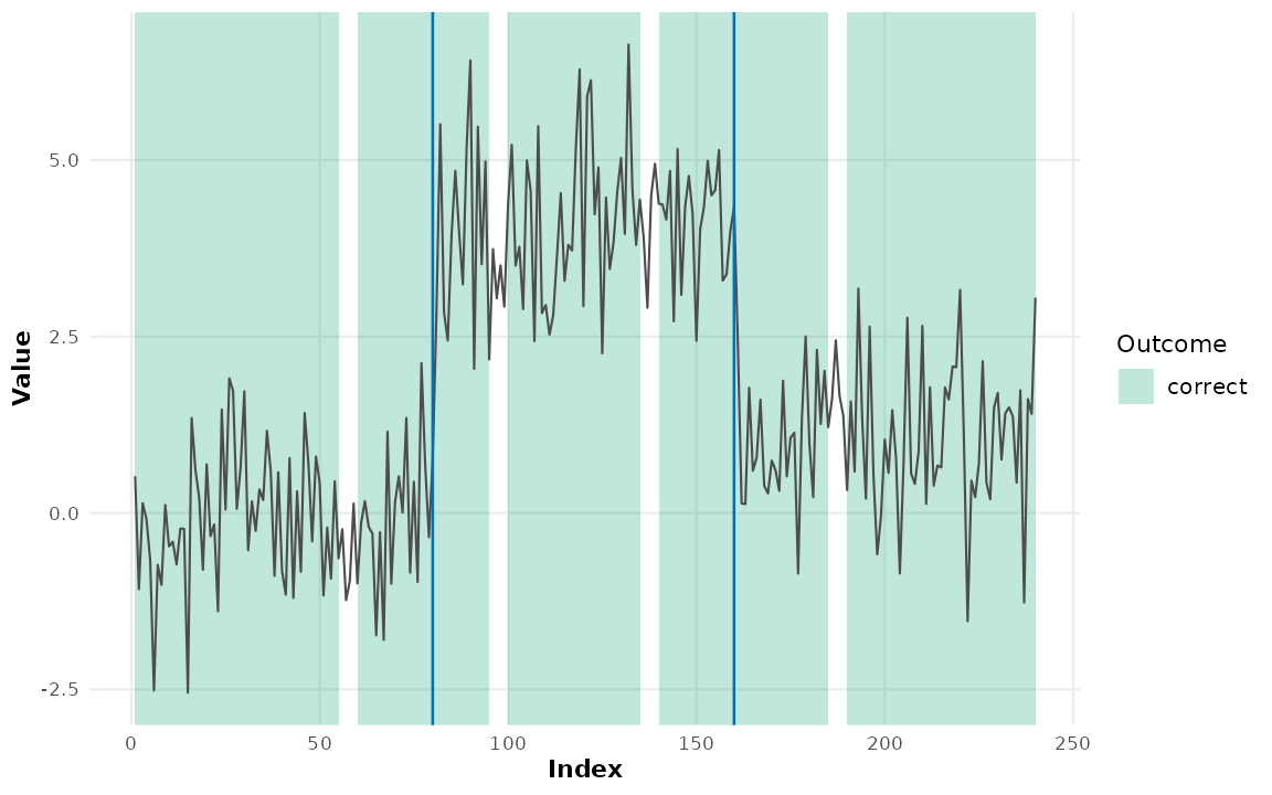

Series with label regions shaded green for correct, orange for false positive and red for false negative

The label error curve

Label errors are a function of the penalty, and the shape of that function is what penalty learning is fitted to. It also answers a question worth asking before any fitting: can any penalty satisfy these labels?

curve <- cpt_label_error_curve(x, labs, method = "pelt")
curve
#> ggcpt_label_curve (method: pelt, 30 penalties)
#>   Minimum label errors: 0
#>   Target log-penalty interval: (2.013, 5.829)
#> 
#> # A tibble: 30 × 5
#>    penalty  n_cp errors false_positive false_negative
#>      <dbl> <int>  <int>          <int>          <int>
#>  1   0.274   147      5              5              0
#>  2   0.353   142      5              5              0
#>  3   0.456   129      5              5              0
#>  4   0.588   115      5              5              0
#>  5   0.758    99      5              5              0
#>  6   0.978    84      5              5              0
#>  7   1.26     66      5              5              0
#>  8   1.63     55      5              5              0
#>  9   2.10     40      5              5              0
#> 10   2.71     26      5              5              0
#> # ℹ 20 more rows

autoplot(curve)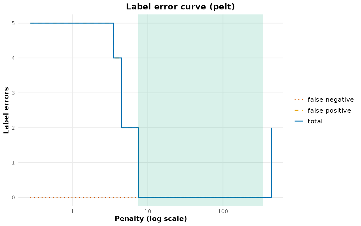

False positives, false negatives and total label errors against the penalty on a log scale, with the target interval shaded

The shaded band is the target interval: the range of log-penalties achieving the minimum error. A wide interval means an easy series; a narrow one means the labels pin the penalty down tightly; an empty minimum at a non-zero error means no penalty satisfies all the labels, and the labels or the method need revisiting.

Learning the penalty

With several labelled series, the target intervals become the response in a max-margin interval regression: features of each series predict a log-penalty that lands inside its interval.

series <- list(
  a = c(rnorm(60), rnorm(60, 4)),
  b = c(rnorm(80), rnorm(80, 2)),
  c = c(rnorm(70), rnorm(70, 6)),
  d = c(rnorm(100, 0, 3), rnorm(100, 9, 3))
)
labels <- list(
  a = as_cpt_labels(60, n = 120),
  b = as_cpt_labels(80, n = 160),
  c = as_cpt_labels(70, n = 140),
  d = as_cpt_labels(100, n = 200)
)
model <- cpt_learn_penalty(series, labels, penalties = 2^(0:10))
model
#> ggcpt_penalty_model (native interval regression)
#>   Trained on 4 series with method `pelt`
#>   Features: log_n, log_log_n, log_sd, log_mad, log_range, log_sd_diff, log_mad_diff, log_q90_abs_diff
#> 
#> Coefficients (predicting log penalty):
#>        intercept            log_n        log_log_n           log_sd 
#>           3.7288          -0.2329          -0.1043           0.3255 
#>          log_mad        log_range      log_sd_diff     log_mad_diff 
#>           0.3358           0.3086           0.2896           0.2788 
#> log_q90_abs_diff 
#>           0.2733 
#> 
#> Use it directly: cpt_detect(x, method = "pelt", penalty = model)

The features are scale-free summaries on the log scale, which is why the fourth series — the same jump measured in units three times as wide — does not simply demand a different penalty from the first.

The model has a predict() method, and — the point of the whole exercise — cpt_detect() takes it wherever a penalty goes:

predict(model, series$d)
#> [1] 347.5184
cpt_detect(series$d, method = "pelt", penalty = model)
#> ggcpt (changepoint detection result)
#>   Method:         pelt
#>   Change in:       mean 
#>   Changepoints found: 1 
#>   CP convention:   left 
#>   Penalty:         Manual = 347.52 
#>   Series length:   200 
#> 
#> Changepoints:
#> # A tibble: 1 × 2
#>      cp cp_value
#>   <int>    <dbl>
#> 1   100     1.77

So does cpt_penalty(), and so do the wrappers that accept a numeric penalty:

cpt_penalty(model, series = series$d)
#> [1] 347.5184

Compare that with the unsupervised default on the same series, which reads its penalty against a raw cost calibrated for unit noise:

nrow(cpt_detect(series$d, method = "pelt")$changepoints)
#> [1] 41
nrow(cpt_detect(series$d, method = "pelt", penalty = model)$changepoints)
#> [1] 1

When is installed, cpt_learn_penalty() delegates the interval regression to IntervalRegressionCV() and keeps the built-in squared-hinge fit as a fallback, so the result is the published estimator whenever the published implementation is available:

cpt_learn_penalty(series, labels, penalties = 2^(0:10),
                  engine = "native")$fit$engine
#> [1] "native"

Where this fits

Labels are annotations, and annotations are also what cpt_metrics_annotated() scores against. They are deliberately the same shape here, so a single set of expert marks can drive the metric, the plot and the penalty. The natural next step is vignette("inference", package = "ggchangepoint"), which covers what to do once the segmentation is fixed.

References

Hocking, Toby Dylan, Guillem Rigaill, Jean-Philippe Vert, and Francis Bach. 2013. “Learning Sparse Penalties for Change-Point Detection Using Max Margin Interval Regression.” Proceedings of the 30th International Conference on Machine Learning 28: 172–80.