How sure is the number of changepoints? Weights over K

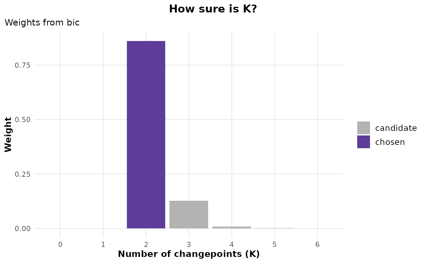
Turns the criterion curve of cpt_select() into weights over the candidate numbers of changepoints, and averages the candidate segmentations under those weights into a probability, at each location, that it is a changepoint.

Usage

cpt_k_weights(sel)

# S3 method for class 'ggcpt_k_weights'
print(x, ...)

# S3 method for class 'ggcpt_k_weights'
tidy(x, what = c("k", "locations"), ...)

# S3 method for class 'ggcpt_k_weights'
glance(x, ...)

# S3 method for class 'ggcpt_k_weights'
autoplot(object, what = c("k", "locations"), ...)

Arguments

sel

A ggcpt_selection from cpt_select() with criterion = "bic", "mbic" or "aic": the criteria on the deviance scale, where weights have their meaning.

x

A ggcpt_k_weights object.

...

Ignored.

what

"k" (default) for the weights, "locations" for the model-averaged location probabilities.

object

A ggcpt_k_weights object.

Value

A ggcpt_k_weights tibble with one row per candidate: k, value (the criterion), delta, weight and chosen. tidy(x, what = "locations") returns the model-averaged probability of a changepoint at each location any candidate uses (position, index, probability); autoplot(x) draws the weights and autoplot(x, what = "locations") the probabilities. print() and glance() (the chosen K, its weight, and the smallest set of K holding 95% of the weight) work on it.

The weights

With \(\Delta_K\) the criterion of \(K\) changepoints minus the smallest, the weight of \(K\) is \(\exp(-\Delta_K / 2)\) normalised over the candidates. For "aic" these are Akaike weights; for "bic" and "mbic" they approximate posterior probabilities of each \(K\) under equal prior weight. They are conditional on the candidate segmentations: each \(K\) is represented by the one segmentation the ladder found for it, so the location probabilities reflect uncertainty about how many changes there are, not about where a given one falls (cpt_confint() answers that).

See also

cpt_select().

Other inference: cpt_abruptness(), cpt_assumptions(), cpt_attribute(), cpt_attribute_event(), cpt_confint_coverage(), cpt_effect(), cpt_gof(), cpt_null_power(), cpt_robustness(), cpt_screen(), cpt_test_at(), cpt_test_null()

Examples

set.seed(2026)
x <- c(rnorm(80), rnorm(80, 1.2), rnorm(80, 0.4))
sel <- cpt_select(x, criterion = "bic", k_max = 6)
w <- cpt_k_weights(sel)
w
#> ggcpt_k_weights (weights over the number of changepoints, from bic)
#>   Chosen:             K = 2, weight 0.861
#>   Largest weights:    K = 2: 0.861; K = 3: 0.128; K = 4: 0.009
#>   95% of the weight:  K in {2, 3}
#> 
#> # A tibble: 7 × 5
#>       k value delta   weight chosen
#>   <int> <dbl> <dbl>    <dbl> <lgl> 
#> 1     0  65.4 48.9  2.10e-11 FALSE 
#> 2     1  31.3 14.7  5.44e- 4 FALSE 
#> 3     2  16.6  0    8.61e- 1 TRUE  
#> 4     3  20.4  3.81 1.28e- 1 FALSE 
#> 5     4  25.6  9.06 9.29e- 3 FALSE 
#> 6     5  29.4 12.9  1.38e- 3 FALSE 
#> 7     6  34.5 17.9  1.12e- 4 FALSE 
tidy(w, what = "locations")
#> # A tibble: 6 × 3
#>   position index probability
#>      <int> <int>       <dbl>
#> 1       15    15    0.0108  
#> 2       37    37    0.00149 
#> 3       76    76    1.000   
#> 4      117   117    0.139   
#> 5      122   122    0.000112
#> 6      161   161    0.999   
ggplot2::autoplot(w)