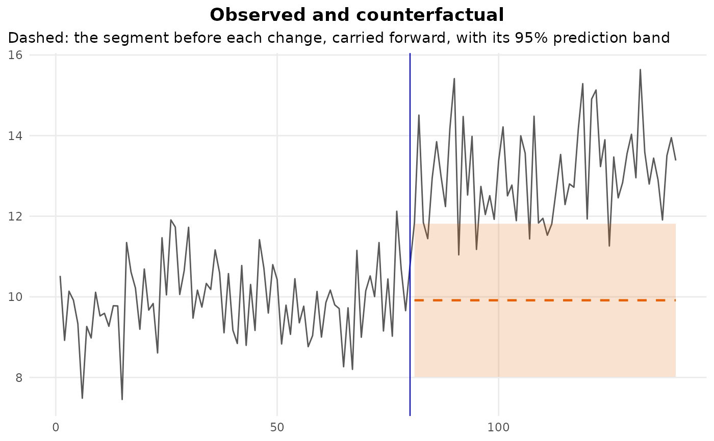
What would have happened without the change? Observed against counterfactual

For each changepoint, carries the segment before it forward over the segment after it, using that segment's own model, and sets the prediction beside what was observed. The gap is the effect of the change, observation by observation, in the units of the data: the interrupted-time-series exhibit.

Usage

cpt_counterfactual(
  fit,
  model = NULL,
  data = NULL,
  engine = stats::lm,
  level = 0.95,
  ...
)

# S3 method for class 'ggcpt_counterfactual'
print(x, ...)

# S3 method for class 'ggcpt_counterfactual'
tidy(x, ...)

# S3 method for class 'ggcpt_counterfactual'
glance(x, ...)

# S3 method for class 'ggcpt_counterfactual'
autoplot(object, ...)

Arguments

fit: A ggcpt object.
model, data, engine, ...: Passed to cpt_segment_models(): the model fitted to each segment (by default its level, its line for a change in slope, or the formula of a formula fit), covariates it uses, and the fitting function.
level: Level of the prediction interval around the counterfactual. Defaults to 0.95.
x: A ggcpt_counterfactual object.
object: A ggcpt_counterfactual object.

Value

A ggcpt_counterfactual tibble with one row per observation after each changepoint, up to the next: cp (the change it belongs to), position, index (the time index, or the position when there is none), observed, counterfactual, lower and upper (the prediction interval, NA when the model supplies none) and effect (observed - counterfactual). autoplot() draws the series with each counterfactual and its band; glance() gives one row per change with the mean and cumulative effect; print() and tidy() work as usual.

Reading it

The counterfactual is a prediction from the pre-change segment alone, so its interval widens the further it is carried: a level is carried at constant width, a line fans out. The interval describes the pre-change model's uncertainty, not the location's: the changepoint is taken as given, and cpt_confint() is the place to ask how sure that location is. Where the detector chose the location from the same data, the effect is the naive one, and cpt_effect() measures it on held-out observations instead.

Examples

set.seed(2026)
x <- c(rnorm(80, 10), rnorm(60, 13))
fit <- cpt_detect(x, method = "pelt", change_in = "meanvar")
cf <- cpt_counterfactual(fit)
glance(cf)
#> # A tibble: 1 × 5
#>      cp     n mean_effect cumulative_effect share_outside
#>   <int> <int>       <dbl>             <dbl>         <dbl>
#> 1    80    60        3.14              188.         0.883
ggplot2::autoplot(cf)