Builds a ladder of candidate segmentations with \(K = 0, 1, \ldots\) changepoints and scores each one, returning the chosen \(K\), the criterion curve behind the choice, and the fitted result at that \(K\). Five criteria are available, including the consistent sample-splitting cross-validation of Zou, Wang and Li (2020) and the segment-length mBIC of Zhang and Siegmund (2007).
Usage
cpt_select(
  x,
  method = "pelt",
  criterion = c("bic", "mbic", "aic", "crops_elbow", "cv", "stability"),
  k_max = 20,
  folds = 5,
  B = 100,
  change_in = "mean",
  index = NULL,
  seed = NULL,
  ...
)

# S3 method for class 'ggcpt_selection'
print(x, ...)

# S3 method for class 'ggcpt_selection'
tidy(x, ...)

# S3 method for class 'ggcpt_selection'
autoplot(
  object,
  plot_type = c("criterion", "segmentation", "ladder"),
  max_facets = 12,
  ...
)
Arguments
- x
A numeric vector, or a
ggcptobject (its series and method are used).- method
Detection method used to build the candidate ladder. Defaults to
"pelt". Taken fromxwhen it is aggcpt. The penalised methods ("pelt","binseg","segneigh","amoc","fpop") give a full nested ladder; the search-based methods tune themselves by an internal criterion and largely ignorepenalty, so their ladder collapses to one or two rungs and the function warns.- criterion
Which criterion selects \(K\):
"bic"Gaussian BIC over the ladder, \(n\log(\mathrm{RSS}/n) + (2K + 1)\log n\). The first term is the Gaussian profile cost reported in the
costcolumn (\(-2\log L\) up to an additive constant, for a common variance); the parameter count is \(K\) locations plus \(K + 1\) segment means. Stated because thevaluecolumn is otherwise not reproducible: both the cost convention and the parameter count vary between authors."mbic"the modified BIC of Zhang and Siegmund (2007), \(3K\log n + \sum_i \log(l_i/n)\) on the deviance (\(-2\log L\)) scale, which is the scale the
costcolumn is on; the same criterion is \(1.5K\log n + 0.5\sum_i \log(l_i/n)\) on the log-likelihood scale, which is howcpt_penalty()states it. It depends on the segment lengths \(l_i\) and so cannot be expressed bycpt_penalty()'s function of \(n\) and \(k\) alone. This is the one place in the package where the real Zhang-Siegmund penalty is computed."aic"Gaussian AIC over the ladder, \(n\log(\mathrm{RSS}/n) + 2(2K + 1)\): the same cost and the same parameter count as
"bic", with \(2\) in place of \(\log n\). That penalty does not grow with \(n\), so it over-selects changepoints, often taking every rung offered: on a 300-point series with changes at 100 and 200,"bic"and"mbic"both choose \(K = 2\) and"aic"chooses the largest \(K\) available. Included because people ask for it and because seeing the curve is instructive;"bic"or"mbic"is the better default."crops_elbow"the knee of the CROPS cost-against-\(K\) curve, made an explicit rule (maximum distance from the chord joining the endpoints, the standard Kneedle construction) rather than something eyeballed off a plot. An elbow needs \(K \ge 1\), so this criterion cannot return \(K = 0\).
"cv"order-preserved sample-splitting cross-validation (COPPS) via crossvalidationCP. This is the criterion with a consistency guarantee. It chooses \(K\) with that package's own least-squares estimator (a change in the mean), not by re-running
method, which then supplies the segmentation at that \(K\). Note thatcpss, the authors' own package, was removed from CRAN; crossvalidationCP is the supportable route."stability"the \(K\) whose changepoints are re-detected most often under within-segment bootstrap resampling. A robustness criterion, not a model-selection one; use it to cross-check the others. It cannot return \(K = 0\).
"bic","mbic"and"cv"can return \(K = 0\);"aic"in principle can and in practice (measured at \(n = 400\)) pickedk_maxor next to it at every true \(K\).cpt_select()warns (classggchangepoint_selection_unadjusted) when"aic"lands at the top of the ladder, and when"crops_elbow"or"stability"returns its smallest candidate.- k_max
Largest number of changepoints considered. Defaults to
20, capped atfloor(n / 4).- folds
Folds for
criterion = "cv". Defaults to5;2gives the original COPPS split.- B
Bootstrap replicates for
criterion = "stability". Defaults to100.- change_in
Passed to the detector, and inherited from
xwhenxis aggcpt(an explicit value still wins). Defaults to"mean".The three closed-form criteria assume a change in the mean whatever this is set to.
"bic","aic"and"mbic"all score the ladder with the Gaussian profile cost \(n\log(\mathrm{RSS}/n)\) (the deviance for a change in mean with a common variance), so on achange_in = "var"ladder the candidates come from the variance detector while the score does not, and splitting a segment whose mean did not move barely reduces \(\mathrm{RSS}\): the criterion will tend to choose \(K = 0\) on a real variance change. Use"stability"there, which scores by re-detection with the samechange_inand so carries no such assumption."cv"does not help: its estimator is a least-squares change in the mean as well.- index
Optional time index (a vector of dates, or a
ts,xts,zooortsibblepassed asx), carried onto the chosen fit sotidy()andautoplot()report the changepoint on your scale rather than as a position. Inherited fromxwhenxis an indexedggcpt.- seed
Optional seed. The seed is scoped to this call:
.Random.seedis saved and restored, so a seeded call inside a simulation loop does not pin the loop's own stream.- ...
Additional arguments passed to
cpt_detect()when the ladder is built by repeated detection.- object
A
ggcpt_selectionobject (forautoplot()).- plot_type
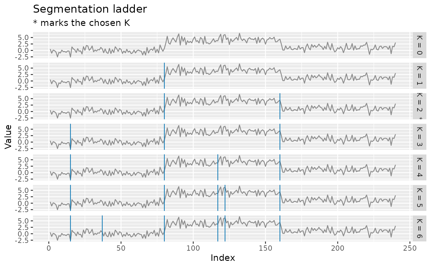
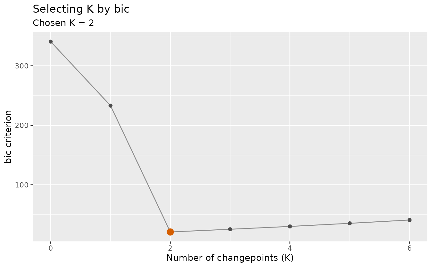
"criterion"(the criterion against \(K\), with the choice marked),"segmentation"(the series with the chosen segmentation) or"ladder"(small multiples showing how the segmentation coarsens as \(K\) falls, the display that makes the choice inspectable rather than asserted).- max_facets
Maximum number of rungs drawn by
plot_type = "ladder". Defaults to12.
Value
A ggcpt_selection object: a list with
criterion_table (one row per candidate \(K\): k,
value, cost, chosen, and a cpts
list-column), k (the chosen number), fit (the
ggcpt at that \(K\)), criterion and data.
Methods: print(), tidy() and autoplot() with
plot_type = "criterion", "segmentation" or
"ladder".
References
Zou C, Wang G, Li R (2020). “Consistent selection of the number of change-points via sample-splitting.” The Annals of Statistics, 48(1), 413–439. doi:10.1214/19-AOS1814 .
Zhang NR, Siegmund DO (2007). “A modified Bayes information criterion with applications to the analysis of comparative genomic hybridization data.” Biometrics, 63(1), 22–32. doi:10.1111/j.1541-0420.2006.00662.x .
Haynes K, Eckley IA, Fearnhead P (2017). “Computationally efficient changepoint detection for a range of penalties.” Journal of Computational and Graphical Statistics, 26(1), 134–143.
Examples
set.seed(2026)
x <- c(rnorm(80), rnorm(80, 4), rnorm(80, 1))
sel <- cpt_select(x, criterion = "bic", k_max = 6)
sel
#> ggcpt_selection (criterion: bic, method: pelt)
#> Candidates scored: K = 0 to 6
#> Chosen K: 2
#> Locations: 80, 160
#>
#> # A tibble: 7 × 4
#> k value cost chosen
#> <int> <dbl> <dbl> <lgl>
#> 1 0 341. 335. FALSE
#> 2 1 233. 217. FALSE
#> 3 2 20.8 -6.60 TRUE
#> 4 3 25.4 -13.0 FALSE
#> 5 4 30.1 -19.2 FALSE
#> 6 5 35.3 -24.9 FALSE
#> 7 6 40.9 -30.3 FALSE
ggplot2::autoplot(sel)
 ggplot2::autoplot(sel, plot_type = "ladder")