Which of many series changed? Screening with error control across the panel

Tests every series in a panel for a change anywhere, with one of cpt_test_null()'s tests, adjusts the p-values across the panel, and returns the series ordered by evidence with the ones that survive flagged. Optionally runs a detector on the flagged series, so the segmentation is spent only where there is something to segment.

Usage

cpt_screen(
  x,
  test = c("pettitt", "cusum", "supF"),
  alpha = 0.05,
  control = c("fdr", "fdr_dependent", "fwer", "none"),
  method = NULL,
  ...
)

# S3 method for class 'ggcpt_screen'
print(x, ...)

# S3 method for class 'ggcpt_screen'
tidy(x, ...)

# S3 method for class 'ggcpt_screen'
glance(x, ...)

# S3 method for class 'ggcpt_screen'
autoplot(object, ...)

Arguments

x

A list of numeric vectors, or a matrix or data frame with one column per series, as for cpt_batch(). For print(), tidy() and glance(), a ggcpt_screen object.

test

Which test gives each series its p-value: "pettitt" (default), "cusum" or "supF"; see cpt_test_null(). Pettitt's rank test is the default because a panel adjustment works in the far tail of each test's null distribution, and there its p-value errs on the safe side while the CUSUM's Kolmogorov limit does not at moderate lengths: measured on panels of 100 series of 120 observations, ten of them with a shift of one standard deviation, the false discovery rate at alpha = 0.05 was 0.030 with Pettitt and 0.065 with the CUSUM, for the same power (0.97 and 0.98; 300 panels). At 500 observations both held (0.039 and 0.052).

alpha

Error level across the panel. Defaults to 0.05.

control

"fdr" (default): Benjamini-Hochberg control of the false discovery rate, valid for independent series (and positively dependent ones); "fdr_dependent": Benjamini and Yekutieli's version, valid under any dependence between series; "fwer": Holm control of the family-wise error rate; "none": no adjustment, which is what running each test on its own amounts to.

method

Optional detection method. When given, every flagged series is segmented with cpt_detect() and the result kept in a result column. Defaults to NULL (screen only).

...

Passed to cpt_detect() when method is given.

object

A ggcpt_screen object, for autoplot().

Value

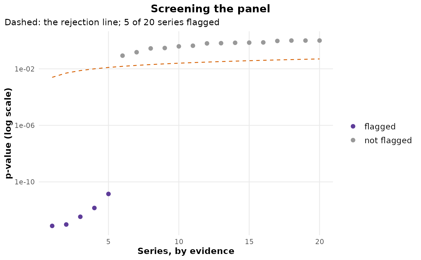
A ggcpt_screen tibble with one row per series, ordered by p-value: series, rank, n, statistic, p_value, p_adjusted, flagged and location (where the test statistic peaks), plus n_changepoints and result (a list-column of ggcpt fits, NULL for series not flagged) when method is given. print(), autoplot() (the sorted p-values against the rejection line), tidy() and glance() work on it.

Why the panel needs its own correction

Each series' p-value is valid for that series. Across a panel of \(m\) stable series, testing each at alpha flags about \(m \alpha\) of them, and nothing in a per-series answer says so. The adjustment is over the series, so its guarantee is about the panel: under "fdr", of the series flagged, the expected share that did not change is at most alpha. The tests assume independent observations within a series, and autocorrelation makes every one of them reject too often; cpt_assumptions() checks a single fit for it.

See also

cpt_batch(), which segments every series and adjusts nothing; cpt_test_null().

Other inference: cpt_abruptness(), cpt_assumptions(), cpt_attribute(), cpt_attribute_event(), cpt_confint_coverage(), cpt_effect(), cpt_gof(), cpt_k_weights(), cpt_null_power(), cpt_robustness(), cpt_test_at(), cpt_test_null()

Examples

set.seed(2026)
panel <- c(lapply(1:15, function(i) rnorm(120)),
           lapply(1:5, function(i) c(rnorm(60), rnorm(60, 1.5))))
names(panel) <- paste0("store", 1:20)
sc <- cpt_screen(panel)
sc
#> ggcpt_screen (pettitt test on each series)
#>   Series:             20
#>   Controls:           false discovery rate (Benjamini-Hochberg) at 0.05
#>   Flagged:            5
#> 
#> # A tibble: 20 × 8
#>    series   rank     n statistic  p_value p_adjusted flagged location
#>    <chr>   <int> <int>     <dbl>    <dbl>      <dbl> <lgl>      <int>
#>  1 store16     1   120      2995 7.70e-14   9.65e-13 TRUE          59
#>  2 store18     2   120      2984 9.65e-14   9.65e-13 TRUE          56
#>  3 store17     3   120      2922 3.41e-13   2.27e-12 TRUE          62
#>  4 store20     4   120      2850 1.42e-12   7.12e-12 TRUE          60
#>  5 store19     5   120      2731 1.40e-11   5.61e-11 TRUE          63
#>  6 store11     6   120       957 8.54e- 2   2.85e- 1 FALSE         57
#>  7 store6      7   120       868 1.49e- 1   4.27e- 1 FALSE         94
#>  8 store10     8   120       757 2.78e- 1   6.57e- 1 FALSE         91
#>  9 store15     9   120       745 2.96e- 1   6.57e- 1 FALSE         25
#> 10 store7     10   120       690 3.88e- 1   7.76e- 1 FALSE         58
#> # ℹ 10 more rows
ggplot2::autoplot(sc)