Detection power for a changepoint scenario

Simulates replicate series under a scenario and reports how often the detector finds the change, how accurately it locates it, and how often it reports changes that are not there. This is the calculation that should precede an analysis, and the one applied papers are increasingly asked for.

Usage

cpt_power(
  n,
  jump,
  sigma = 1,
  method = "pelt",
  location = 0.5,
  n_sim = 200,
  tolerance = 5,
  change_in = "mean",
  noise = "gauss",
  rho = 0,
  df = 3,
  seed = NULL,
  parallel = TRUE,
  ...
)

# S3 method for class 'ggcpt_power'
tidy(x, ...)

# S3 method for class 'ggcpt_power'
print(x, ...)

# S3 method for class 'ggcpt_power'
autoplot(object, ...)

Arguments

n

Series length.

jump

Size of the change, in units of sigma. A vector runs one scenario per value.

sigma

Noise standard deviation. Defaults to 1.

method

Detection method. Defaults to "pelt".

location

Changepoint position, as a fraction of n in \((0, 1)\) or an integer position. Defaults to 0.5. A vector runs one scenario per value.

n_sim

Replicates per scenario. Defaults to 200.

tolerance

A detection counts as finding the change when it falls within this many positions of it. Defaults to 5.

change_in

What changes. Defaults to "mean".

noise

Noise model, passed to cpt_simulate().

rho

AR(1) parameter when noise = "ar1".

df

Degrees of freedom when noise = "t".

seed

Optional seed.

parallel

Use future::plan() when future.apply is available? Defaults to TRUE.

...

Additional arguments passed to cpt_detect().

x

A ggcpt_power object.

object

A ggcpt_power object (for autoplot()).

Value

A ggcpt_power object: a tibble with one row per scenario — n, jump, sigma, location, power (proportion of replicates detecting the change within tolerance), mc_se (the Monte Carlo standard error of that proportion), mean_abs_error (location error among detections), false_positive_rate (mean number of extra changepoints per replicate) and n_sim — with print() and autoplot().

See also

cpt_min_detectable(), cpt_scenarios(), cpt_simulate().

Examples

# \donttest{
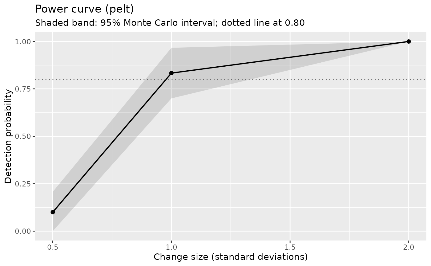
pw <- cpt_power(n = 200, jump = c(0.5, 1, 2), n_sim = 30, seed = 1)
pw
#> ggcpt_power (method: pelt, change in mean, gauss noise, tolerance 5)
#>   3 scenario(s), 30 replicates each
#> 
#> # A tibble: 3 × 9
#>       n  jump sigma location power  mc_se mean_abs_error false_positive_rate
#>   <int> <dbl> <dbl>    <int> <dbl>  <dbl>          <dbl>               <dbl>
#> 1   200   0.5     1      100 0.1   0.0548          2.67                0.1  
#> 2   200   1       1      100 0.833 0.0680          1.32                0.167
#> 3   200   2       1      100 1     0               0.467               0    
#> # ℹ 1 more variable: n_sim <int>
#> 
#> Monte Carlo standard errors are in `mc_se`; a power of 0.80 from 30
#> replicates is only known to about +/- 0.14.
ggplot2::autoplot(pw)

# }