Sensitivity of a segmentation to its tuning parameters

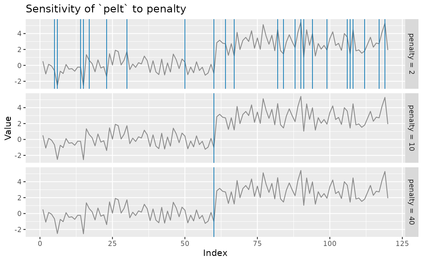
The parameter analogue of cpt_influence(): instead of asking which observation drives the answer, it asks which setting does. Runs the detector over a grid of tuning values and reports the detected locations for each, which is the direct answer to the commonest reviewer question about a changepoint analysis — "is this robust to the penalty?".

Usage

cpt_sensitivity(x, method = "pelt", over = list(), seed = NULL, ...)

# S3 method for class 'ggcpt_sensitivity'
print(x, ...)

# S3 method for class 'ggcpt_sensitivity'
tidy(x, ...)

# S3 method for class 'ggcpt_sensitivity'
autoplot(object, ...)

Arguments

x

A numeric vector (the series), or a ggcpt object, in which case its series and method are used.

method

Detection method. Taken from x when it is a ggcpt.

over

A named list of parameter vectors to sweep. Every combination is run, so keep the grid small: list(penalty = c(5, 10, 20), minseglen = c(2, 10)).

seed

Optional seed.

...

Additional arguments held fixed across the grid and passed to cpt_detect().

object

A ggcpt_sensitivity object (for autoplot()).

Value

A ggcpt_sensitivity object: a list with a grid tibble (one row per setting: the parameter columns, n_cp, and a cpts list-column), the data, and the swept parameter names. Methods: print(), tidy() (one row per detected changepoint) and autoplot() (a location heatmap over the grid).

See also

cpt_influence(), cpt_select().

Examples

set.seed(2026)
x <- c(rnorm(60), rnorm(60, 3))
s <- cpt_sensitivity(x, method = "pelt",
                     over = list(penalty = c(2, 10, 40)))
s
#> ggcpt_sensitivity (method: pelt, 3 settings)
#>   Swept: penalty
#>   Changepoints found: 1 to 24
#> 
#> # A tibble: 3 × 2
#>   penalty  n_cp
#>     <dbl> <int>
#> 1       2    24
#> 2      10     1
#> 3      40     1
ggplot2::autoplot(s)