Benchmark detectors across datasets

Runs a grid of methods over a collection of labelled series and scores every cell with cpt_metrics() (or cpt_metrics_annotated() when a dataset carries several annotators). An engine that errors on one dataset records the message and the grid continues.

Usage

cpt_benchmark(
  datasets,
  methods = c("pelt", "binseg", "wbs"),
  metrics = c("covering", "f1"),
  tolerance = 5,
  change_in = "mean",
  parallel = TRUE,
  progress = TRUE,
  seed = NULL,
  ...
)

# S3 method for class 'ggcpt_benchmark'
print(x, ...)

# S3 method for class 'ggcpt_benchmark'
tidy(x, ...)

# S3 method for class 'ggcpt_benchmark'
autoplot(
  object,
  plot_type = c("heatmap", "ranks", "critical_difference"),
  metric = NULL,
  alpha = 0.05,
  ...
)

Arguments

datasets: A named list of datasets. Each element is either a plain numeric vector (no ground truth, so only descriptive columns are filled) or a list with series and one of truth, changepoints (an integer vector) or annotations (a list of integer vectors, one per annotator). A list carrying none of those is scored NA and warns. A series with several columns stays a matrix, so only the multivariate methods can score it. cpt_datasets() builds a ready-made collection.
methods: Character vector of method names.
metrics: Which metrics to keep. Defaults to c("covering", "f1"), the pair van den Burg and Williams (2020) established as the benchmark standard.
tolerance: Matching window passed to the metrics. Defaults to 5.
change_in: Passed to every detector.
parallel: Use future::plan() when future.apply is available? Defaults to TRUE.
progress: Show a progressr progress bar when that package is installed and a handler is enabled? Defaults to TRUE.
seed: Optional seed. The seed is scoped to this call: .Random.seed is saved and restored, so a seeded call inside a simulation loop does not pin the loop's own stream.
...: Additional arguments passed to every cpt_detect() call.
x: A ggcpt_benchmark object.
object: A ggcpt_benchmark object (for autoplot()).
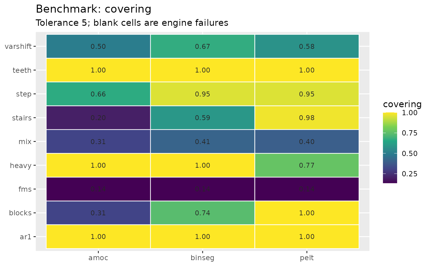
plot_type: "heatmap" (method by dataset, coloured by the metric), "ranks" (mean rank per method) or "critical_difference" (the Demšar diagram: mean ranks with the Nemenyi critical distance, the standard way this literature says "method A beats method B").
metric: Which metric to plot. Defaults to the first one scored.
alpha: Level for the critical distance, in (0, 1). Defaults to 0.05. Only used by plot_type = "critical_difference", which also needs at least two methods to compare.

Value

A ggcpt_benchmark object: a tibble with one row per (dataset, method): dataset, method, n, n_annotators (how many ground-truth sets the dataset supplied), n_cp, the requested metrics, runtime and error, with print(), tidy() and autoplot() ("heatmap", "ranks", "critical_difference").

Reading the critical-difference diagram

Rank 1 is best. Each method's mean rank is taken over the datasets, in the direction the metric calls for: higher is better for covering, f1, precision, recall and rand_index; lower for hausdorff, annotation_error, mae_matched and rmse_matched. A metric that came back NA takes the worst rank on that dataset rather than being dropped, so a method that failed there is penalised for it instead of quietly scoring on a smaller sample; ties share the average rank.

The bar is the Nemenyi critical distance $$CD = q_\alpha \sqrt{k(k + 1) / (6N)}$$ for $k$ methods over $N$ datasets, where $q_\alpha$ is the Studentised range statistic at $\alpha$ divided by $\sqrt 2$ (Demsar, 2006; the constants agree with that paper's Table 5 to three decimals for $k = 2, \ldots, 10$). Two methods whose mean ranks differ by less than $CD$ are not distinguished at that level.

One caveat the diagram cannot show. Nemenyi is a post-hoc procedure, and the convention is to run it only after a Friedman test has rejected the null that all methods rank equally. autoplot() does not run that omnibus test (it draws the diagram it is asked for), so a gap wider than $CD$ on a grid where Friedman would not have rejected is not the significant difference it looks like. With the handful of datasets cpt_datasets() supplies, $N$ is small and $CD$ correspondingly wide; read the diagram as a descriptive summary unless $N$ is large enough to support the test.

References

van den Burg GJJ, Williams CKI (2020). “An evaluation of change point detection algorithms.” arXiv preprint arXiv:2003.06222. doi:10.48550/arXiv.2003.06222 .

Demšar J (2006). “Statistical comparisons of classifiers over multiple data sets.” Journal of Machine Learning Research, 7, 1–30.

Examples

# \donttest{
bm <- cpt_benchmark(cpt_datasets(n = 200, seed = 1),
                    methods = c("pelt", "binseg", "amoc"),
                    progress = FALSE)
#> Warning: The number of changepoints identified is Q, it is advised to increase Q to make sure changepoints have not been missed.
#> Warning: The number of changepoints identified is Q, it is advised to increase Q to make sure changepoints have not been missed.
#> Warning: The number of changepoints identified is Q, it is advised to increase Q to make sure changepoints have not been missed.
bm
#> ggcpt_benchmark (9 dataset(s) x 3 method(s), tolerance 5)
#> 
#> Mean rank across datasets (1 = best):
#> # A tibble: 3 × 4
#>   method mean_rank n_datasets n_datasets_total
#>   <chr>      <dbl>      <int>            <int>
#> 1 binseg      1.67          9                9
#> 2 pelt        1.83          9                9
#> 3 amoc        2.5           9                9
#> 
#> # A tibble: 27 × 4
#>    dataset  method covering    f1
#>    <chr>    <chr>     <dbl> <dbl>
#>  1 blocks   pelt      1     1    
#>  2 fms      pelt      0.135 0    
#>  3 mix      pelt      0.396 0    
#>  4 teeth    pelt      1     1    
#>  5 stairs   pelt      0.980 1    
#>  6 step     pelt      0.952 1    
#>  7 ar1      pelt      1     1    
#>  8 heavy    pelt      0.77  0.5  
#>  9 varshift pelt      0.577 0    
#> 10 blocks   binseg    0.739 0.625
#> 11 fms      binseg    0.135 0    
#> 12 mix      binseg    0.413 0    
#> # ℹ 15 more rows
ggplot2::autoplot(bm)

# }