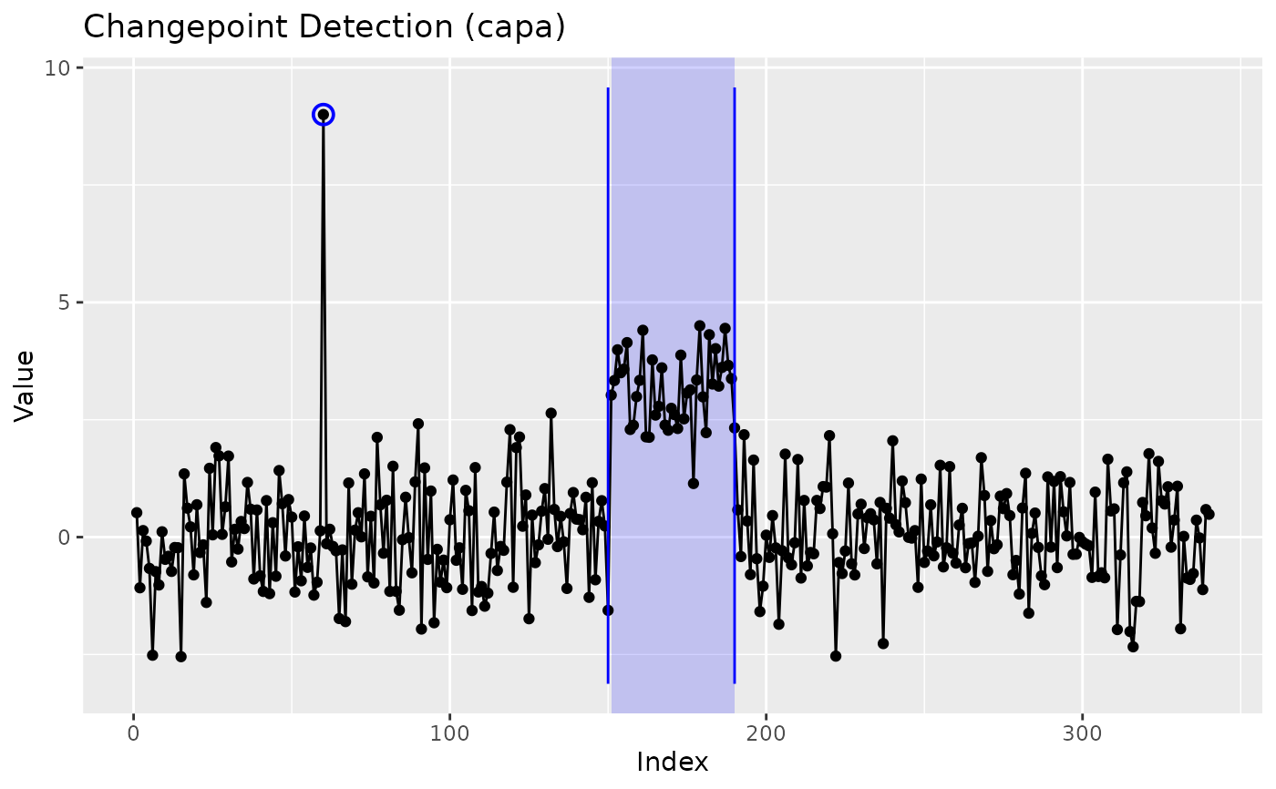
CAPA wrapper: collective and point anomalies (epidemic changepoints)

Wraps anomaly::capa() (Fisch, Eckley and Fearnhead 2022): finds stretches of the series that depart from a persistent baseline and return to it (collective anomalies: an outbreak that subsides, a fault that is repaired, a campaign that ends) and single outlying observations (point anomalies), for one series or many. For a multivariate series it also reports which coordinates each anomaly affects.

Usage

capa_wrapper(
  x,
  change_in = c("mean", "meanvar"),
  robust = FALSE,
  beta = NULL,
  beta_tilde = NULL,
  min_seg_len = 10,
  max_seg_len = Inf,
  max_lag = 0,
  standardise = TRUE,
  ...
)

Arguments

x

A numeric vector, or a matrix or data frame with one column per coordinate.

change_in

"mean" (default) for anomalies in the mean, "meanvar" for anomalies in mean and variance.

robust

For change_in = "mean" on a single series, use CAPA's robust cost (type = "robustmean"), which tolerates outliers inside an anomalous stretch. Defaults to FALSE.

beta

Penalty for a collective anomaly: one number, or one per coordinate. NULL (default) uses the engine's own penalty.

beta_tilde

Penalty for a point anomaly. NULL (default) uses the engine's 3 log(np).

min_seg_len

Shortest collective anomaly, at least 2. Defaults to 10, the engine's default.

max_seg_len

Longest collective anomaly. Defaults to Inf.

max_lag

For a multivariate series, how far an anomaly's start and end may differ between coordinates. Defaults to 0.

standardise

Centre and scale each coordinate by its median and median absolute deviation before the search. Defaults to TRUE. CAPA assumes a baseline of mean 0 and variance 1, so leave this on unless the data are already on that scale.

...

Not used; present so the dispatcher can pass its own arguments through. Anything supplied is refused by name.

Value

A ggcpt object whose changepoints are the anomaly boundaries and whose regions slot lists the anomalies, plus a baseline element holding the centre and scale used to standardise each coordinate.

How the result reads

The baseline is everything that is not anomalous, and it is one regime, which is what separates this model from an ordinary segmentation. Each collective anomaly from s to e contributes two changepoints, s - 1 (the last baseline observation before it) and e (its last observation), so the segments alternate between the baseline and the anomalies and every tool built on changepoints works unchanged. The anomalies themselves are in the regions slot, read with cpt_regions(): one row per anomaly with start, end, type ("collective" or "point"), coordinates (the affected coordinates, comma separated), mean_change (the engine's squared standardised mean change for a collective anomaly) and strength (the engine's strength for a point anomaly). Point anomalies are outliers, not changes, so they add no changepoint. autoplot() shades the collective anomalies and rings the point ones, and cpt_attribute() can certify, with error control, which coordinates changed at each boundary.

A series whose two halves differ, with no baseline to return to, is not what CAPA models: the median of such a series lies between the two levels, so both halves look anomalous. Use an ordinary detector for a step.

References

Fisch ATM, Eckley IA, Fearnhead P (2022). “A linear time method for the detection of collective and point anomalies.” Statistical Analysis and Data Mining, 15(4), 494–508. doi:10.1002/sam.11586 .

Fisch ATM, Eckley IA, Fearnhead P (2022). “Subset multivariate collective and point anomaly detection.” Journal of Computational and Graphical Statistics, 31(2), 574–585. doi:10.1080/10618600.2021.1987257 .

See also

cpt_regions(), cpt_attribute().

Other changepoint engines: bcp_wrapper(), beast_wrapper(), bfast_wrapper(), binsegrcpp_wrapper(), bocpd_wrapper(), cpm_wrapper(), cpop_wrapper(), cpt_wrapper(), decafs_wrapper(), ecp_wrapper(), envcpt_wrapper(), esac_wrapper(), fabisearch_wrapper(), fastcpd_wrapper(), fcov_wrapper(), fmean_wrapper(), fpop_wrapper(), geomcp_wrapper(), hdcov_wrapper(), hdreg_wrapper(), idetect_wrapper(), inspect_wrapper(), kcp_wrapper(), kwc_wrapper(), mcp_wrapper(), mosum_wrapper(), network_wrapper(), not_wrapper(), npmojo_wrapper(), nsp_wrapper(), ocd_wrapper(), pilliat_wrapper(), segmented_wrapper(), smuce_wrapper(), sn_wrapper(), strucchange_wrapper(), taylor_wrapper(), tguh_wrapper(), trend_wrapper(), var_wrapper(), wbs2_wrapper(), wbs_wrapper(), wbsts_wrapper()

Examples

set.seed(2026)
x <- c(rnorm(150), rnorm(40, 3), rnorm(150))
x[60] <- 9
fit <- capa_wrapper(x)
cpt_regions(fit)
#> # A tibble: 2 × 7
#>   start   end length type       coordinates mean_change strength
#>   <int> <int>  <int> <chr>      <chr>             <dbl>    <dbl>
#> 1    60    60      1 point      V1                NA        7.39
#> 2   151   190     40 collective V1                 6.16    NA   
ggplot2::autoplot(fit)