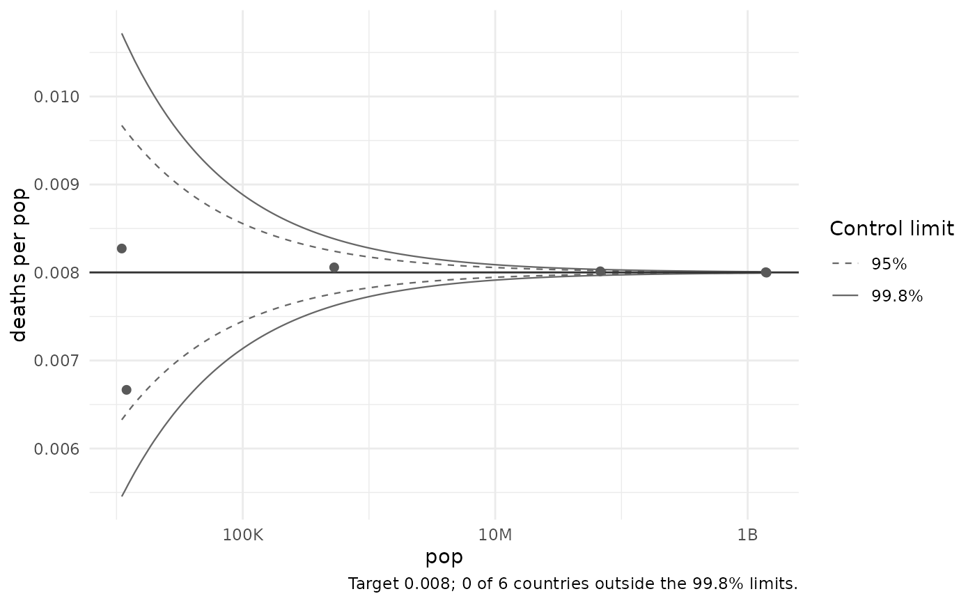
Each country's rate against its denominator, inside control limits for the
rate a country of that size would show by chance alone. A small country's
extreme rate falls inside the wide mouth of the funnel; a large country
outside the narrow neck is a real outlier. It completes the rates set:
rate_check() flags the unreliable rates, smooth_rates() shrinks them,
rate_funnel() shows them, value_by_alpha_map() maps them.
Usage
rate_funnel(
  data,
  numerator,
  denominator,
  target = NULL,
  limits = c(0.95, 0.998),
  overdispersion = FALSE,
  label_outliers = TRUE
)
Arguments
- data
A country-level frame with
iso3c.- numerator, denominator
The counts and their population at risk (unquoted).
- target
The rate the limits are drawn around;
NULL(default) is the pooled rate,sum(numerator) / sum(denominator).- limits
The coverage of the inner and outer limits (default
c(0.95, 0.998), Spiegelhalter's "two and three sigma").- overdispersion
If
TRUE, widen the limits by the additive random-effects adjustment (Spiegelhalter 2005), for rates that vary between countries far more than Poisson noise allows – the usual case for country data, where a funnel with exact limits flags most countries.- label_outliers
Label the countries outside the outer limit with their ISO code (default
TRUE).
Value
A ggplot, with the per-country table attached as the
"countryatlas_funnel" attribute: iso3c, the two columns, rate, z
(the standardised deviation) and flag ("within", "above 95%",
"above 99.8%", "below 95%" or "below 99.8%", named after limits).
The limits
For a denominator \(d\) the expected count is \(E = t d\), and the
limit at probability \(P\) is the exact Poisson quantile, interpolated
so the funnel is smooth: with \(r = F^{-1}(P; E)\),
\(y_P = r - (F(r; E) - P) / (F(r; E) - F(r - 1; E))\), and the rate limit
is \(y_P / d\). With overdispersion = TRUE the limits are
\(t \pm z_P \sqrt{t / d + \tau^2}\), \(\tau^2\) estimated from the
winsorised z-scores.
References
Spiegelhalter, D. J. (2005). Funnel plots for comparing institutional performance. Statistics in Medicine 24(8), 1185-1202. doi:10.1002/sim.1970