Spatial statistics on a world of islands

A spatial statistic is only as good as its idea of who is next to whom. On a world map, land borders leave Japan, Australia, New Zealand and every island state with no neighbours at all, so a statistic on contiguity weights silently drops a quarter of the countries with data. The package defaults to the five nearest neighbours, so every country with a centroid takes part.

knn <- morans_i(snap, gdp_per_capita, n_perm = 499)
border <- morans_i(snap, gdp_per_capita, n_perm = 499,
                   weights = country_weights("contiguity"))
rbind(knn = knn[, c("i", "n", "n_excluded", "p_value")],
      contiguity = border[, c("i", "n", "n_excluded", "p_value")])
#> # A tibble: 2 × 4
#>       i     n n_excluded p_value
#> * <dbl> <int>      <int>   <dbl>
#> 1 0.452   199          0   0.002
#> 2 0.600   146         53   0.002

Local clusters, with the false discoveries controlled

A local Moran test runs once per country, so about one in twenty comes out “significant” by chance at the 5% level. local_morans() and lisa_map() control the false discovery rate by default (Caldas de Castro & Singer 2006), on 9,999 conditional permutations so the smallest p-values can clear it.

lisa_map(attach_geometry(snap), gdp_per_capita, n_perm = 999)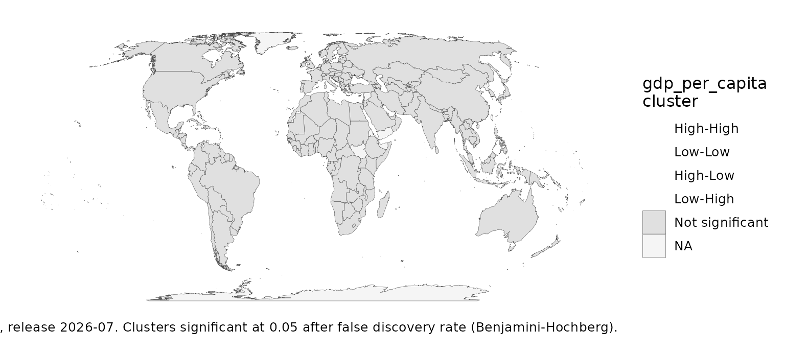

Two variables at once: high GDP per capita among long-lived neighbours.

b <- bivariate_lisa(snap, gdp_per_capita, life_expectancy, n_perm = 999)
table(b$cluster)
#> 
#>       High-High         Low-Low        High-Low        Low-High Not significant 
#>               9              29               0               0             161

Rates

Moran’s I on raw rates mistakes the noise of small denominators for clustering. eb_morans_i() standardises each rate by its own reliability first (Assuncao & Reis 1999); it agrees with spdep::EBImoran.mc().

set.seed(2)
d <- snap[!is.na(snap$population), ]
d$births <- stats::rpois(nrow(d), d$population * 0.018)
eb_morans_i(d, births, population, n_perm = 499)
#> # A tibble: 1 × 7
#>         i expected     n n_excluded n_links p_value excluded 
#>     <dbl>    <dbl> <int>      <int>   <int>   <dbl> <list>   
#> 1 -0.0451 -0.00467   215          1     979   0.816 <chr [1]>

Categories and dynamics

Do income groups cluster? Join counts compare the neighbouring pairs in the same group with random labelling:

join_counts(snap, income, n_perm = 499)
#> # A tibble: 5 × 7
#>   category                n joins expected    sd     z p_value
#>   <chr>               <int> <int>    <dbl> <dbl> <dbl>   <dbl>
#> 1 High income            80   146    84.9   6.64  9.20   0.002
#> 2 Low income             26    33     8.66  2.60  9.37   0.002
#> 3 Lower middle income    54    65    38.2   5.35  5.02   0.002
#> 4 Not classified          1     0     0     0    NA      1    
#> 5 Upper middle income    54    61    38.3   5.08  4.46   0.002

spatial_markov() asks whether a country’s neighbours change its odds of moving between classes (Rey 2001), with a homogeneity test; see ?spatial_markov.