
The headline use case: I have a frame keyed on messy country names; get it on a map. The package exposes the same matching machinery it uses internally.
Standardise any frame
standardize_country() attaches ISO codes and
classifications, reconciling spellings automatically:
my_data <- data.frame(
  nation = c("U.S.", "S. Korea", "Czechia", "Kosovo", "Cote d'Ivoire", "UK"),
  score  = c(10, 8, 6, 4, 7, 9)
)
standardize_country(my_data, nation, warn = FALSE)
#> # A tibble: 6 × 6
#>   nation        score iso3c iso2c continent region
#>   <chr>         <dbl> <chr> <chr> <chr>     <chr>
#> 1 U.S.             10 USA   US    Americas  North America
#> 2 S. Korea          8 KOR   KR    Asia      East Asia & Pacific
#> 3 Czechia           6 CZE   CZ    Europe    Europe & Central Asia
#> 4 Kosovo            4 XKX   XK    Europe    Europe & Central Asia
#> 5 Cote d'Ivoire     7 CIV   CI    Africa    Sub-Saharan Africa
#> 6 UK                9 GBR   GB    Europe    Europe & Central Asia
One call to a map
join_world() auto-detects the country column,
standardises it and attaches geometry:
my_data |>
  join_world(nation, warn = FALSE) |>
  world_map(score, title = "My data on the ISO spine")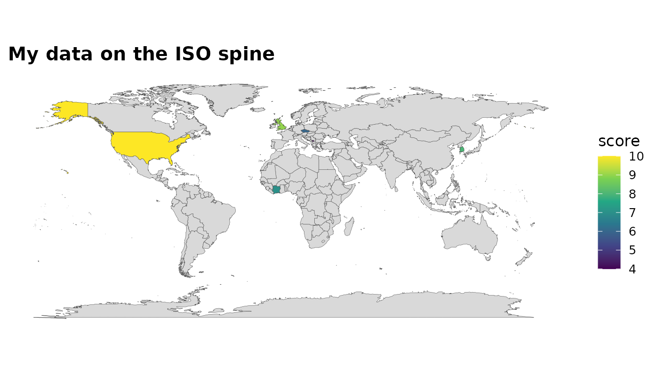
Reconcile two messy tables
country_join() joins two frames that each key on country
names, by reconciling both sides to iso3c first:
a <- data.frame(country = c("Czechia", "South Korea", "Russia"), gdp = 1:3)
b <- data.frame(nation  = c("Czech Republic", "Korea, Rep.", "Russian Federation"),
                pop = c(10, 51, 144))
country_join(a, b, country, nation)
#> # A tibble: 3 × 5
#>   country       gdp iso3c nation               pop
#>   <chr>       <int> <chr> <chr>              <dbl>
#> 1 Czechia         1 CZE   Czech Republic        10
#> 2 South Korea     2 KOR   Korea, Rep.           51
#> 3 Russia          3 RUS   Russian Federation   144
Reconcile many tables at once
country_join_all() generalises this to a whole list of
frames: every table is reconciled to iso3c first, then
reduce-joined, so three sources spelled three ways collapse into one
honest table:
t1 <- data.frame(country = c("Czechia", "South Korea"), gdp = c(1, 2))
t2 <- data.frame(country = c("Czech Republic", "Korea, Rep."), pop = c(10, 51))
t3 <- data.frame(country = c("Czechia", "Korea"), area = c(79, 100))
country_join_all(list(t1, t2, t3), by = "country")
#> # A tibble: 2 × 7
#>   country.x     gdp iso3c country.y        pop country  area
#>   <chr>       <dbl> <chr> <chr>          <dbl> <chr>   <dbl>
#> 1 Czechia         1 CZE   Czech Republic    10 Czechia    79
#> 2 South Korea     2 KOR   Korea, Rep.       51 Korea     100
Check before you trust
Always inspect what failed to match:
check_country_match(my_data$nation)
#> # A tibble: 6 × 6
#>   input         iso3c matched historical method   suggestion
#>   <chr>         <chr> <lgl>   <lgl>      <chr>    <chr>
#> 1 U.S.          USA   TRUE    FALSE      regex_en NA
#> 2 S. Korea      KOR   TRUE    FALSE      regex_en NA
#> 3 Czechia       CZE   TRUE    FALSE      regex_en NA
#> 4 Kosovo        XKX   TRUE    FALSE      override NA
#> 5 Cote d'Ivoire CIV   TRUE    FALSE      regex_en NA
#> 6 UK            GBR   TRUE    FALSE      regex_en NA
Historical data: dissolved countries
Historical panels bring a nastier failure mode: dissolved entities.
Most are silently unmatched, but some are silently mismatched.
countrycode resolves "USSR" to Russia’s RUS,
so Soviet-era totals quietly become Russian totals. The
historical column in the report above flags both cases, and
dissolve_country() resolves them to successor states via
the curated historical_codes crosswalk (one row per
successor, dated):
check_country_match(c("USSR", "Yugoslavia", "West Germany"))
#> # A tibble: 3 × 6
#>   input        iso3c matched historical method   suggestion
#>   <chr>        <chr> <lgl>   <lgl>      <chr>    <chr>
#> 1 USSR         RUS   TRUE    TRUE       regex_en NA
#> 2 Yugoslavia   NA    FALSE   TRUE       none     Yugoslavia
#> 3 West Germany DEU   TRUE    FALSE      regex_en NA
dissolve_country(c("Czechoslovakia", "France"))
#> # A tibble: 3 × 5
#>   input          historical     dissolved iso3c country
#>   <chr>          <chr>              <int> <chr> <chr>
#> 1 Czechoslovakia Czechoslovakia      1993 CZE   Czechia
#> 2 Czechoslovakia Czechoslovakia      1993 SVK   Slovakia
#> 3 France         NA                    NA FRA   France
"West Germany" is the instructive case: it resolves to
DEU and is not flagged, correctly so, because the
Federal Republic never dissolved. It absorbed the GDR in 1990 and simply
continued, so DEU really is the right answer. The crosswalk
is curated rather than a blanket rule that anything old-sounding gets
flagged, so only the entity that actually ceased to exist is listed:
historical_codes maps East Germany (DDR) to
DEU.
Repair what can be repaired
repair_country_names() is the “act on it” companion to
that report: it substitutes the closest known country name, but only
when the match is confident, and attaches a record of what it
changed:
fixed <- repair_country_names(c("Brzil", "Nehterlands", "United States"),
                              verbose = FALSE)
fixed
#> [1] "Brazil"        "Netherlands"   "United States"
#> attr(,"repairs")
#> # A tibble: 2 × 2
#>   from        to
#>   <chr>       <chr>
#> 1 Brzil       Brazil
#> 2 Nehterlands Netherlands
If something legitimately cannot be matched (an entity the backends simply do not know), extend the override table:
country_overrides(c(Somaliland = "SOM"))[c("Kosovo", "Somaliland")]
#>     Kosovo Somaliland
#>      "XKX"      "SOM"
Custom origins
If your key is already an ISO-2 or World Bank code, tell
standardize_country() via origin:
df <- data.frame(code = c("US", "KR", "BR"))
standardize_country(df, code, origin = "iso2c", warn = FALSE)
#> # A tibble: 3 × 5
#>   code  iso3c iso2c continent region
#>   <chr> <chr> <chr> <chr>     <chr>
#> 1 US    USA   US    Americas  North America
#> 2 KR    KOR   KR    Asia      East Asia & Pacific
#> 3 BR    BRA   BR    Americas  Latin America & Caribbean
Point data onto the spine
Not all data comes keyed on names; sometimes all you have is
coordinates (events, weather stations, survey sites).
locate_country() runs a point-in-polygon lookup and tags
each point with the country that contains it, so point data joins the
ISO spine like everything else. It needs the optional sf +
rnaturalearth packages:
locate_country(lon = c(2.35, -74.0, 139.7), lat = c(48.85, 40.7, 35.7))
#> # A tibble: 3 × 2
#>   iso3c country
#>   <chr> <chr>
#> 1 FRA   France
#> 2 USA   United States
#> 3 JPN   Japan
Coarse coastlines can place a genuinely-onshore point (a port city,
say) just outside its country’s simplified polygon;
locate_country() snaps such points to the nearest country
within tolerance_km (25 km by default) while leaving
open-ocean points NA.