countryatlas: Joining World Data to Maps on the ISO Spine

Abstract

Joining country-level data across independent sources is deceptively hard: the same country is spelled "US", "U.S.", "United States" and "United States of America", and a naïve join treats them as different entities. countryatlas resolves this friction by adopting ISO 3166 codes as a universal join key and by stitching together three otherwise disjoint resources — map geometry, World Bank development indicators, and a comprehensive country-code crosswalk — into a single, map-ready table. This vignette presents the package’s design philosophy, its complete functional vocabulary, and worked examples spanning data assembly, the join engine, diagnostics, reference data, analysis helpers and a full grammar of honest cartographic displays. All examples run offline against a bundled data snapshot.

Introduction

The package rests on a single conviction: if a task does not make it easier to get country data onto a map — or to make that map honest — it does not belong here. Concretely, three packages are combined:

ggplot2::map_data("world") (or Natural Earth via sf) supplies polygon geometry, i.e. where countries are;
WDI supplies World Bank indicators, i.e. what is true about them;
countrycode supplies the crosswalk of ISO codes, continents and regions that makes a reliable join possible.

Three design commitments follow. First, the happy path is one call: world_data(2020) returns a tibble ready to map. Second, the ISO code is the spine: every function speaks iso3c/iso2c internally and exposes it, so anything the package produces joins to anything else — and to the user’s own data. Third, no country is lost silently: entities that map backends spell idiosyncratically are matched through a curated override table rather than dropped, and unmatched values are reported explicitly.

To keep every example reproducible without a network connection, this vignette uses the bundled world_snapshot dataset, a curated set of indicators for one recent year.

snapshot <- world_snapshot$countries
dplyr::glimpse(snapshot)
#> Rows: 215
#> Columns: 10
#> $ iso3c           <chr> "AFG", "ALB", "DZA", "ASM", "AND", "AGO", "ATG", "ARG"…
#> $ iso2c           <chr> "AF", "AL", "DZ", "AS", "AD", "AO", "AG", "AR", "AM", …
#> $ country         <chr> "Afghanistan", "Albania", "Algeria", "American Samoa",…
#> $ continent       <chr> "Asia", "Europe", "Africa", "Oceania", "Europe", "Afri…
#> $ region          <chr> "South Asia", "Europe & Central Asia", "Middle East & …
#> $ income          <fct> Low income, Upper middle income, Upper middle income, …
#> $ gdp_per_capita  <dbl> NA, 6549.234, 4765.729, NA, 41034.527, 2845.478, 18350…
#> $ population      <dbl> 42647492, 2377128, 46814308, 46765, 81938, 37885849, 9…
#> $ life_expectancy <dbl> 66.28900, 79.77600, 76.47500, 72.99200, 84.18800, 64.8…
#> $ co2_per_capita  <dbl> 0.282980298, 1.785221494, 3.980800058, 0.002138351, NA…

Core data assembly

`world_data()`

The headline function is generalised but backward-compatible. The classic call returns the polygon-backed, enriched tibble exactly as before:

# Live World Bank API call (not evaluated here to keep the vignette offline):
world_data(2020)
world_data(
  2020,
  indicator = c(life_exp = "SP.DYN.LE00.IN", co2 = "EN.GHG.CO2.PC.CE.AR5"),
  geometry  = "sf",
  region    = "Africa"
)

The indicator argument accepts one or many WDI codes; a named vector drives clean column names. A range of years (2000:2020) yields a panel keyed on iso3c and year. The geometry argument switches between the classic "polygon" backend, a modern "sf" backend with real projections, and "none" for pure analysis.

`country_data()` and `attach_geometry()`

For analysis you usually want one tidy row per country, not ~99,000 polygon vertices. country_data() provides exactly that, and geometry is attached only at draw time:

mapdf <- attach_geometry(snapshot, geometry = "polygon")
dim(mapdf)
#> [1] 99338    15

Visualising: the choropleth and beyond

One-line choropleths

world_map() encapsulates the plotting boilerplate and offers several honest styles. A continuous fill on a skewed indicator hides most of the variation, so binned and quantile styles are first-class:

world_map(mapdf, gdp_per_capita, style = "quantile",
          title = "GDP per capita (quantile bins)")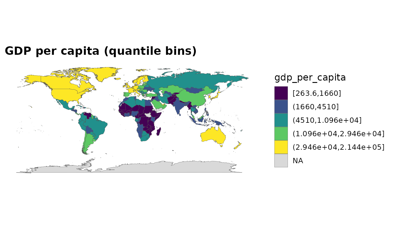

world_map(mapdf, continent, style = "categorical")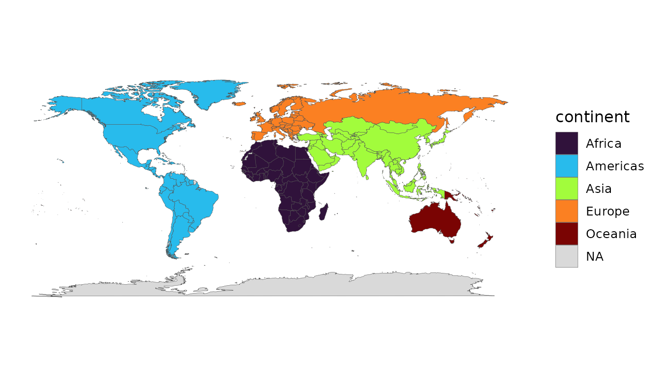

Proportional-symbol maps

Totals (population, total emissions) are misrepresented by a choropleth because large values hide in small countries. A bubble map at country centroids is the right idiom:

bubble_map(snapshot, population)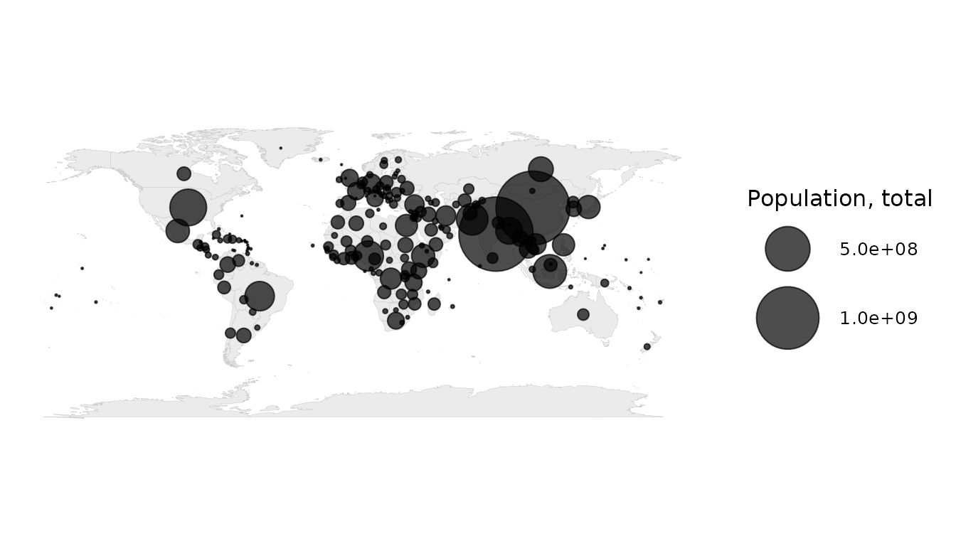

Equal-area tile grids

Tiny states vanish on a geographic map. An equal-area tile grid gives every country the same visual weight:

tile_map(snapshot, life_expectancy)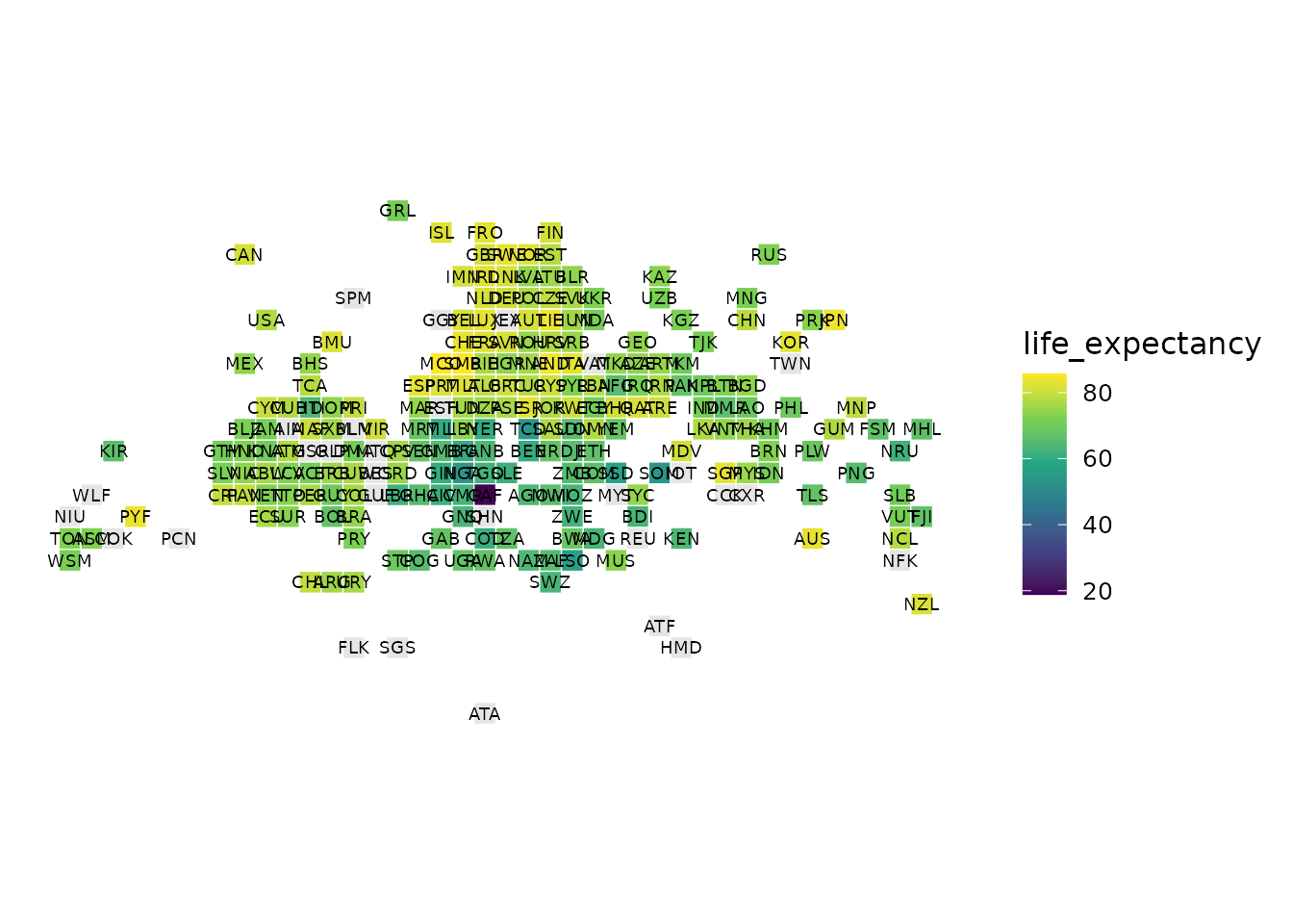

Flow maps

Origin–destination data (trade, migration, flights) is drawn as great-circle arcs, with both endpoints resolved to centroids automatically:

flows <- data.frame(
  from   = c("China", "Germany", "Brazil", "India"),
  to     = c("United States", "France", "Japan", "United Kingdom"),
  weight = c(500, 200, 150, 120)
)
flow_map(flows, from, to, weight)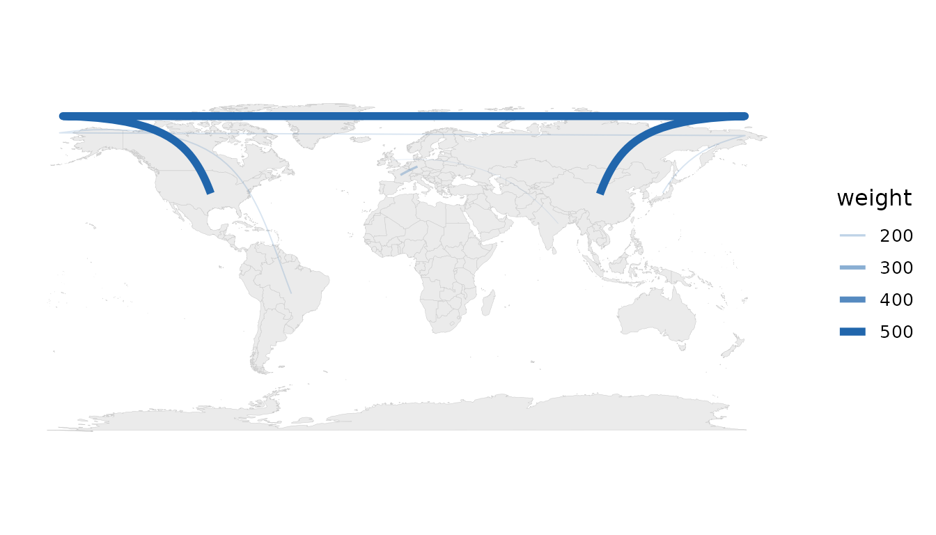

The join engine

The package’s mission, exposed for the reader’s own data. Given a frame keyed on messy names, standardize_country() attaches ISO codes and classifications:

messy <- data.frame(
  nation = c("U.S.", "S. Korea", "Czechia", "Kosovo", "Cote d'Ivoire"),
  value  = c(10, 8, 6, 4, 7)
)
standardize_country(messy, nation, warn = FALSE)
#> # A tibble: 5 × 6
#>   nation        value iso3c iso2c continent region               
#>   <chr>         <dbl> <chr> <chr> <chr>     <chr>                
#> 1 U.S.             10 USA   US    Americas  North America        
#> 2 S. Korea          8 KOR   KR    Asia      East Asia & Pacific  
#> 3 Czechia           6 CZE   CZ    Europe    Europe & Central Asia
#> 4 Kosovo            4 XKX   XK    Europe    Europe & Central Asia
#> 5 Cote d'Ivoire     7 CIV   CI    Africa    Sub-Saharan Africa

join_world() goes one step further — auto-detecting the country column, standardising it and attaching geometry — while country_join() reconciles two independent tables that each key on country names:

left  <- data.frame(country = c("Czechia", "South Korea"), gdp = c(1, 2))
right <- data.frame(nation  = c("Czech Republic", "Korea, Rep."), pop = c(10, 51))
country_join(left, right, country, nation)
#> # A tibble: 2 × 5
#>   country       gdp iso3c nation           pop
#>   <chr>       <dbl> <chr> <chr>          <dbl>
#> 1 Czechia         1 CZE   Czech Republic    10
#> 2 South Korea     2 KOR   Korea, Rep.       51

Diagnostics: never lose a country silently

check_country_match() is a pre-flight report; country_overrides() is the curated match table that replaces the old drop-list; and audit_coverage() reports missingness before a half-empty map is published.

check_country_match(c("USA", "Cote d'Ivoire", "Yugoslavia", "Wakanda"))
#> # A tibble: 4 × 5
#>   input         iso3c matched historical suggestion
#>   <chr>         <chr> <lgl>   <lgl>      <chr>     
#> 1 USA           USA   TRUE    FALSE      NA        
#> 2 Cote d'Ivoire CIV   TRUE    FALSE      NA        
#> 3 Yugoslavia    NA    FALSE   TRUE       Yugoslavia
#> 4 Wakanda       NA    FALSE   FALSE      Canada

repair_country_names() acts on that report: it substitutes the closest known country name for confident misses only, and attaches a record of every change:

repair_country_names(c("Brzil", "Germny", "United States"), verbose = FALSE)
#> [1] "Brazil"        "Germany"       "United States"
#> attr(,"repairs")
#> # A tibble: 2 × 2
#>   from   to     
#>   <chr>  <chr>  
#> 1 Brzil  Brazil 
#> 2 Germny Germany

audit_coverage(snapshot)$na_rates
#> # A tibble: 4 × 4
#>   indicator           n n_missing na_rate
#>   <chr>           <int>     <int>   <dbl>
#> 1 gdp_per_capita    215        24  0.112 
#> 2 population        215         0  0     
#> 3 life_expectancy   215         0  0     
#> 4 co2_per_capita    215        12  0.0558

The entities the previous version dropped — Kosovo, Micronesia, the Virgin Islands and a dozen others — are now matched:

dropped <- c("Kosovo", "Micronesia", "Virgin Islands", "Canary Islands",
             "Saint Martin")
standardize_country(data.frame(region = dropped), region, warn = FALSE)
#> # A tibble: 5 × 4
#>   iso3c iso2c continent region                   
#>   <chr> <chr> <chr>     <chr>                    
#> 1 XKX   XK    Europe    Europe & Central Asia    
#> 2 FSM   FM    Oceania   East Asia & Pacific      
#> 3 VIR   VI    Americas  Latin America & Caribbean
#> 4 ESP   ES    Europe    Europe & Central Asia    
#> 5 MAF   MF    Americas  Latin America & Caribbean

Dissolved entities get first-class treatment too. The historical column of check_country_match() flags them — including "USSR", which countrycode silently resolves to Russia’s RUS (so Soviet-era data becomes Russian data without a warning) — and dissolve_country() expands them to their successor states via the curated historical_codes crosswalk:

check_country_match(c("USSR", "Czechoslovakia"))
#> # A tibble: 2 × 5
#>   input          iso3c matched historical suggestion    
#>   <chr>          <chr> <lgl>   <lgl>      <chr>         
#> 1 USSR           RUS   TRUE    TRUE       NA            
#> 2 Czechoslovakia NA    FALSE   TRUE       Czechoslovakia
dissolve_country("Yugoslavia")
#> # A tibble: 7 × 5
#>   input      historical dissolved iso3c country             
#>   <chr>      <chr>          <int> <chr> <chr>               
#> 1 Yugoslavia Yugoslavia      1992 BIH   Bosnia & Herzegovina
#> 2 Yugoslavia Yugoslavia      1992 HRV   Croatia             
#> 3 Yugoslavia Yugoslavia      1992 MKD   North Macedonia     
#> 4 Yugoslavia Yugoslavia      1992 MNE   Montenegro          
#> 5 Yugoslavia Yugoslavia      1992 SRB   Serbia              
#> 6 Yugoslavia Yugoslavia      1992 SVN   Slovenia            
#> 7 Yugoslavia Yugoslavia      1992 XKX   Kosovo

Reference data and code translation

convert_country() exposes the full countrycode vocabulary with first-class shortcuts for the high-value schemes:

convert_country(c("Japan", "Brazil", "Germany"), to = "flag")
#> [1] "🇯🇵" "🇧🇷" "🇩🇪"
convert_country(c("Japan", "Brazil", "Germany"), to = "currency")
#> [1] "JPY" "BRL" "EUR"

Country-group membership is a curated, dated table:

country_groups("G7")
#> # A tibble: 7 × 3
#>   group iso3c country       
#>   <chr> <chr> <chr>         
#> 1 G7    CAN   Canada        
#> 2 G7    FRA   France        
#> 3 G7    DEU   Germany       
#> 4 G7    ITA   Italy         
#> 5 G7    JPN   Japan         
#> 6 G7    GBR   United Kingdom
#> 7 G7    USA   United States
in_group(c("France", "United States", "Japan", "Brazil"), "EU")
#> [1]  TRUE FALSE FALSE FALSE

The whole countrycode codelist is exposed as a tidy, pipeable lookup with country_codes(), and the World Bank indicator catalogue is searchable offline with wdi_search():

head(country_codes(c("continent", "currency")))
#> # A tibble: 6 × 4
#>   country        iso3c continent currency
#>   <chr>          <chr> <chr>     <chr>   
#> 1 Afghanistan    AFG   Asia      AFN     
#> 2 Albania        ALB   Europe    ALL     
#> 3 Algeria        DZA   Africa    DZD     
#> 4 American Samoa ASM   Oceania   USD     
#> 5 Andorra        AND   Europe    EUR     
#> 6 Angola         AGO   Africa    AOA
head(wdi_search("renewable energy"), 3)
#> # A tibble: 3 × 2
#>   indicator                    name                                     
#>   <chr>                        <chr>                                    
#> 1 2.1_SHARE.TOTAL.RE.IN.TFEC   Renewable energy consumption(% in TFEC)  
#> 2 3.1_RE.CONSUMPTION           Renewable energy consumption (TJ)        
#> 3 4.1.2_REN.ELECTRICITY.OUTPUT Renewable energy electricity output (GWh)

The package also bundles country_meta (static per-country attributes), common_indicators (a friendly indicator catalogue), country_groups_tbl and world_tiles.

Analysis helpers

Small, in-spirit transforms that keep an analysis from leaving the package mid-pipeline:

snapshot |>
  rank_countries(gdp_per_capita) |>
  filter(rank <= 5) |>
  select(country, gdp_per_capita, rank, percentile)
#> # A tibble: 5 × 4
#>   country     gdp_per_capita  rank percentile
#>   <chr>                <dbl> <int>      <dbl>
#> 1 Bermuda            122118.     2      0.995
#> 2 Ireland             94475.     4      0.984
#> 3 Luxembourg         104147.     3      0.989
#> 4 Monaco             247170.     1      1    
#> 5 Switzerland         90067.     5      0.979

snapshot |>
  aggregate_regions(population, by = "region", fun = "sum")
#> # A tibble: 8 × 2
#>   region                     population
#>   <chr>                           <dbl>
#> 1 East Asia & Pacific        2364906595
#> 2 Europe & Central Asia       926500729
#> 3 Latin America & Caribbean   658983093
#> 4 Middle East & North Africa  519229480
#> 5 North America               381464223
#> 6 South Asia                 1971301188
#> 7 Sub-Saharan Africa         1291044964
#> 8 NA                            3203295

For panel data, growth_rate() (year-on-year or CAGR), index_to() (rebase a series so the base year = 100) and share_of_world() (share of the year’s world total) cover the standard comparative moves, each computed per country:

panel <- data.frame(
  iso3c = rep(c("USA", "CHN"), each = 3),
  year  = rep(2019:2021, 2),
  gdp   = c(100, 104, 109, 60, 66, 73)
)
panel |>
  growth_rate(gdp) |>
  index_to(gdp, base_year = 2019)
#> # A tibble: 6 × 5
#>   iso3c  year   gdp gdp_growth gdp_index
#>   <chr> <int> <dbl>      <dbl>     <dbl>
#> 1 CHN    2019    60    NA           100 
#> 2 CHN    2020    66     0.100       110 
#> 3 CHN    2021    73     0.106       122.
#> 4 USA    2019   100    NA           100 
#> 5 USA    2020   104     0.0400      104 
#> 6 USA    2021   109     0.0481      109

And complete_years() fills the panel gaps that would otherwise make an animation flicker or a join silently drop years — by grid completion, carry-forward or linear interpolation (lag_by_country() and diff_by_country() round out the panel toolkit):

patchy <- data.frame(iso3c = "USA", year = c(2019L, 2021L), gdp = c(100, 110))
complete_years(patchy, 2019:2021, method = "linear")
#> # A tibble: 3 × 3
#>   iso3c  year   gdp
#>   <chr> <int> <dbl>
#> 1 USA    2019   100
#> 2 USA    2020   105
#> 3 USA    2021   110

Inequality, correlation and convergence

Three questions this data is constantly asked: how unequal is the world, what moves together, and are poor countries catching up? gini() and theil() measure inequality across countries — weight by population and they describe inequality between people; theil() decomposes exactly into between/within components:

gini(snapshot$gdp_per_capita, weights = snapshot$population)
#> [1] 0.6094909
theil(snapshot$gdp_per_capita, weights = snapshot$population,
      groups = snapshot$continent)
#> # A tibble: 3 × 3
#>   component value share
#>   <chr>     <dbl> <dbl>
#> 1 total     0.678 1    
#> 2 between   0.310 0.458
#> 3 within    0.368 0.542

correlate_indicators() screens indicator pairs (pairwise-complete, with the per-pair n reported so a correlation computed on 12 countries cannot masquerade as a world fact):

correlate_indicators(snapshot)
#> # A tibble: 6 × 4
#>   var_x           var_y                  r     n
#>   <chr>           <chr>              <dbl> <int>
#> 1 gdp_per_capita  life_expectancy  0.607     191
#> 2 gdp_per_capita  co2_per_capita   0.435     184
#> 3 life_expectancy co2_per_capita   0.307     203
#> 4 gdp_per_capita  population      -0.0579    191
#> 5 population      life_expectancy -0.0188    215
#> 6 population      co2_per_capita   0.00660   203

For panels, beta_convergence() runs the classic growth-on-initial-level regression (returning the implied convergence speed and half-life) and sigma_convergence() tracks whether cross-country dispersion is actually narrowing. And on the spatial side, morans_i() measures whether neighbouring countries have similar values, using the package’s own country_borders() adjacency — no spdep needed.

Performance and offline use

World Bank fetches are memoised with an optional on-disk cache, and multiple indicators are fetched in parallel where the platform supports forking. The bundled world_snapshot makes every example here run without the network. The cache can be cleared with clear_wdi_cache().

Conclusion

countryatlas keeps its original soul — ISO codes as the universal join key, one call to a map-ready table — and extends it into a complete toolkit: any indicator and any year span, a modern sf backend, an exposed join engine for the user’s own data, honest diagnostics, curated reference data, analysis helpers, and a full vocabulary of projected, area-honest maps.

Session information

sessionInfo()
#> R version 4.6.1 (2026-06-24)
#> Platform: x86_64-pc-linux-gnu
#> Running under: Ubuntu 24.04.4 LTS
#> 
#> Matrix products: default
#> BLAS:   /usr/lib/x86_64-linux-gnu/openblas-pthread/libblas.so.3 
#> LAPACK: /usr/lib/x86_64-linux-gnu/openblas-pthread/libopenblasp-r0.3.26.so;  LAPACK version 3.12.0
#> 
#> locale:
#>  [1] LC_CTYPE=C.UTF-8       LC_NUMERIC=C           LC_TIME=C.UTF-8       
#>  [4] LC_COLLATE=C.UTF-8     LC_MONETARY=C.UTF-8    LC_MESSAGES=C.UTF-8   
#>  [7] LC_PAPER=C.UTF-8       LC_NAME=C              LC_ADDRESS=C          
#> [10] LC_TELEPHONE=C         LC_MEASUREMENT=C.UTF-8 LC_IDENTIFICATION=C   
#> 
#> time zone: UTC
#> tzcode source: system (glibc)
#> 
#> attached base packages:
#> [1] stats     graphics  grDevices utils     datasets  methods   base     
#> 
#> other attached packages:
#> [1] dplyr_1.2.1        ggplot2_4.0.3      countryatlas_2.0.0
#> 
#> loaded via a namespace (and not attached):
#>  [1] tidyr_1.3.2        sass_0.4.10        utf8_1.2.6         generics_0.1.4    
#>  [5] class_7.3-23       KernSmooth_2.23-26 digest_0.6.39      magrittr_2.0.5    
#>  [9] countrycode_1.8.0  evaluate_1.0.5     grid_4.6.1         RColorBrewer_1.1-3
#> [13] fastmap_1.2.0      maps_3.4.3         jsonlite_2.0.0     e1071_1.7-17      
#> [17] purrr_1.2.2        viridisLite_0.4.3  scales_1.4.0       stringdist_0.9.17 
#> [21] textshaping_1.0.5  jquerylib_0.1.4    cli_3.6.6          rlang_1.3.0       
#> [25] withr_3.0.3        cachem_1.1.0       yaml_2.3.12        otel_0.2.0        
#> [29] tools_4.6.1        parallel_4.6.1     memoise_2.0.1      vctrs_0.7.3       
#> [33] R6_2.6.1           proxy_0.4-29       lifecycle_1.0.5    classInt_0.4-11   
#> [37] fs_2.1.0           htmlwidgets_1.6.4  ragg_1.5.2         pkgconfig_2.0.3   
#> [41] desc_1.4.3         pkgdown_2.2.1      pillar_1.11.1      bslib_0.11.0      
#> [45] gtable_0.3.6       glue_1.8.1         systemfonts_1.3.2  xfun_0.60         
#> [49] tibble_3.3.1       tidyselect_1.2.1   knitr_1.51         farver_2.1.2      
#> [53] htmltools_0.5.9    rmarkdown_2.31     labeling_0.4.3     compiler_4.6.1    
#> [57] WDI_2.7.10         S7_0.2.2