Introduction to tidyEmoji

Youzhi Yu
University of Chicago

Overview

Emoji are everywhere in modern text — social-media posts, product reviews, chat and support logs, survey free-text — and they carry information that plain words do not. Yet summarising emoji from a corpus is surprisingly awkward. Unicode does not interact cleanly with regular expressions, not every code point is an emoji, and a single visible emoji is often built from several code points joined together. Counting “how many posts contain an emoji” or “which emoji are most common” by hand quickly becomes painful.

tidyEmoji removes that friction. It provides a small family of verbs that take a data frame and the name of a text column, and return tidy data frames that drop straight into a dplyr/ggplot2 workflow:

Task	Function(s)
Summarise / filter	emoji_summary(), emoji_filter()
Extract	emoji_extract_nest(), emoji_extract_unnest(), emoji_tokens()
Count	emoji_frequency(), top_n_emojis()
Categorise	emoji_categorize()
Score sentiment	emoji_sentiment()
Score emotions	emoji_emotion(), emoji_emotion_label()
Custom lexicons	emoji_lexicons(), register_emoji_lexicon(), emoji_score()
Translate	emoji_to_text(), text_to_emoji(), as_emoji*()
Search	emoji_search()
Relate	emoji_pairs(), emoji_cooccurrence(), emoji_ngrams()
Measure	emoji_position(), emoji_density(), emoji_ratio()
Interpretation risk	emoji_ambiguity(), emoji_risk(), emoji_flag_ambiguous()
Context	emoji_context(), emoji_collocations()
Functional type	emoji_type(), emoji_faceness(), as_emoji_type()
Time	emoji_trend(), emoji_turnover(), emoji_seasonality(), emoji_version_profile(), emoji_adoption_lag()
Text-emoji mismatch	emoji_incongruity(), emoji_congruence(), emoji_incongruity_profile()
Model features	emoji_dfm()
LLM pipelines	emoji_sanitize(), emoji_token_cost()
Provenance	emoji_provenance(), emoji_unicode_version(), emoji_unicode_releases()

Two design choices are worth highlighting:

• Grapheme-aware detection. Detection is performed on whole grapheme clusters, so skin-tone modifiers (👍🏽) and zero-width-joiner sequences such as the family emoji (👨‍👩‍👧‍👦) are treated as a single emoji rather than being split into their component parts. This is illustrated in the extraction section.
• Tidy by default. Every verb returns a tibble, follows the verb(data, text_column) convention, and supports unquoted column names, so the functions compose naturally with the pipe.

library(tidyEmoji)
library(dplyr)
library(ggplot2)

Example data

Throughout this vignette we use a sample of text collected in Atlanta, Georgia. The data happens to come from a social-media corpus, but nothing below is specific to any platform — any data frame with a text column will do.

ata_tweets <- readr::read_csv("ata_tweets.csv", show_col_types = FALSE)
ata_tweets
#> # A tibble: 2,000 × 1
#>    full_text                                                                    
#>    <chr>                                                                        
#>  1 "Was Justin Bieber ever at any BLM March/protest this past summer? Or ever?" 
#>  2 "Whole Family gone and I’m stuck here in Brunswick 😭"                       
#>  3 "38 years old and I still get distracted while cleaning my room. \n\nJust in…
#>  4 "This time last year I was blasting fever nonstop by Wizkid 😭"              
#>  5 "Kanye is a just a black man with a lot of confidence and y’all tear him dow…
#>  6 "Feel like being my inner self today"                                        
#>  7 "Peep toe boots irk my sole."                                                
#>  8 "Nah the biggest naruto fans be trying call one piece long like... nigga?"   
#>  9 "if my shoes don’t arrive by next Friday imma be pissed"                     
#> 10 "Phone dry asf 🙄"                                                           
#> # ℹ 1,990 more rows

The actual text lives in the full_text column, which is the column we pass to each tidyEmoji verb.

Detecting and summarising emoji

emoji_summary()

emoji_summary() answers the first question one usually asks of a new corpus: how much emoji is in here? It returns a one-row tibble with the number of entries that contain at least one emoji and the total number of entries. An entry is counted once regardless of how many emoji it holds.

summary_tbl <- ata_tweets %>%
  emoji_summary(full_text)

summary_tbl
#> # A tibble: 1 × 2
#>   n_with_emoji n_total
#>          <int>   <int>
#> 1          560    2000

Here, 560 of the 2,000 entries (28%) contain at least one emoji.

emoji_filter()

emoji_filter() keeps only the rows whose text contains at least one emoji, preserving every original column. This is useful when you want to compare emoji-bearing and emoji-free text, or restrict an analysis to the emoji subset. (emoji_tweets() is a synonym retained for backward compatibility.)

ata_tweets %>%
  emoji_filter(full_text)
#> # A tibble: 560 × 1
#>    full_text                                                                    
#>    <chr>                                                                        
#>  1 Whole Family gone and I’m stuck here in Brunswick 😭                         
#>  2 This time last year I was blasting fever nonstop by Wizkid 😭                
#>  3 Phone dry asf 🙄                                                             
#>  4 When I gave my life to Christ, I was able to see people as imperfect, but st…
#>  5 Everyone needs self care days❤️                                               
#>  6 R u sears rn 🤦🏽‍♀️                                                              
#>  7 Gucci wit some dope runnas head huncho top gunna u a sto runna😭             
#>  8 i’m thinking insomnia cause they got this caramel apple pie cookie. 😋       
#>  9 i deadass listen to the music everyday lmao🥲                                
#> 10 Im ona block where ya barley can be at  if you try get shot down 😈          
#> # ℹ 550 more rows

Extracting emoji

tidyEmoji offers three complementary ways to pull the emoji out of text, depending on the shape of output you want.

emoji_extract_nest()

emoji_extract_nest() leaves the data unchanged except for an added list-column, .emoji_unicode, holding the emoji found in each row. The original data structure is preserved, which makes this convenient as an intermediate step.

ata_tweets %>%
  emoji_extract_nest(full_text) %>%
  select(full_text, .emoji_unicode)
#> # A tibble: 2,000 × 2
#>    full_text                                                      .emoji_unicode
#>    <chr>                                                          <list>        
#>  1 "Was Justin Bieber ever at any BLM March/protest this past su… <chr [0]>     
#>  2 "Whole Family gone and I’m stuck here in Brunswick 😭"         <chr [1]>     
#>  3 "38 years old and I still get distracted while cleaning my ro… <chr [0]>     
#>  4 "This time last year I was blasting fever nonstop by Wizkid 😭… <chr [1]>     
#>  5 "Kanye is a just a black man with a lot of confidence and y’a… <chr [0]>     
#>  6 "Feel like being my inner self today"                          <chr [0]>     
#>  7 "Peep toe boots irk my sole."                                  <chr [0]>     
#>  8 "Nah the biggest naruto fans be trying call one piece long li… <chr [0]>     
#>  9 "if my shoes don’t arrive by next Friday imma be pissed"       <chr [0]>     
#> 10 "Phone dry asf 🙄"                                             <chr [1]>     
#> # ℹ 1,990 more rows

emoji_extract_unnest()

emoji_extract_unnest() returns a long, tidy table with one row per (entry, emoji) pair: .row_number records the position of the entry in the data, .emoji_unicode is the emoji, and .emoji_count is how many times that emoji occurs in that entry. Entries without emoji are dropped.

emoji_per_tweet <- ata_tweets %>%
  emoji_extract_unnest(full_text)

emoji_per_tweet
#> # A tibble: 696 × 3
#>    .row_number .emoji_unicode .emoji_count
#>          <int> <chr>                 <int>
#>  1           2 😭                        1
#>  2           4 😭                        1
#>  3          10 🙄                        1
#>  4          15 😂                        1
#>  5          17 ❤️                         1
#>  6          30 🤦🏽‍♀️                        1
#>  7          31 😭                        1
#>  8          33 😋                        1
#>  9          42 🥲                        1
#> 10          45 😈                        1
#> # ℹ 686 more rows

We can use this to plot how many emoji each emoji-bearing entry contains:

emoji_per_tweet %>%
  group_by(.row_number) %>%
  summarise(n_emoji = sum(.emoji_count)) %>%
  ggplot(aes(n_emoji)) +
  geom_bar() +
  scale_x_continuous(breaks = seq(1, 15)) +
  labs(x = "Number of emoji in the entry",
       y = "Number of entries",
       title = "Most emoji-bearing entries contain a single emoji")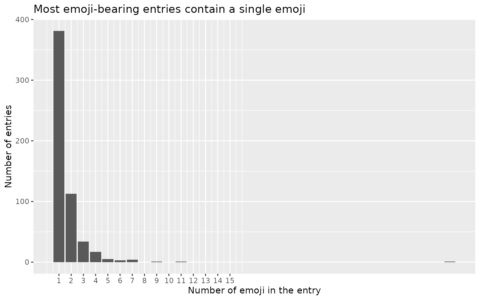

The overwhelming majority of emoji-bearing entries carry just one emoji, with a long, thin tail of more emoji-heavy entries.

emoji_tokens()

emoji_tokens() produces a “one row per emoji occurrence” table — the emoji analogue of a tidy-text token table. It keeps the original columns and adds the glyph (.emoji) together with its name (.emoji_name), category (.emoji_category) and sentiment score (.emoji_sentiment). This single call gives you everything needed for counting, joining and plotting.

ata_tweets %>%
  emoji_tokens(full_text)
#> # A tibble: 900 × 5
#>    full_text                 .emoji .emoji_name .emoji_category .emoji_sentiment
#>    <chr>                     <chr>  <chr>       <chr>                      <dbl>
#>  1 Whole Family gone and I’… 😭     loudly cry… Smileys & Emot…          -0.0934
#>  2 This time last year I wa… 😭     loudly cry… Smileys & Emot…          -0.0934
#>  3 Phone dry asf 🙄          🙄     face with … Smileys & Emot…          NA     
#>  4 When I gave my life to C… 😂     face with … Smileys & Emot…           0.221 
#>  5 Everyone needs self care… ❤️      red heart   Smileys & Emot…           0.746 
#>  6 R u sears rn 🤦🏽‍♀️           🤦🏽‍♀️     woman face… People & Body            NA     
#>  7 Gucci wit some dope runn… 😭     loudly cry… Smileys & Emot…          -0.0934
#>  8 i’m thinking insomnia ca… 😋     face savor… Smileys & Emot…           0.634 
#>  9 i deadass listen to the … 🥲     smiling fa… Smileys & Emot…          NA     
#> 10 Im ona block where ya ba… 😈     smiling fa… Smileys & Emot…           0.268 
#> # ℹ 890 more rows

A note on grapheme-aware detection

Modern emoji are frequently composed of several code points: a base emoji plus a skin-tone modifier, or several emoji joined by zero-width joiners. tidyEmoji detects emoji at the level of grapheme clusters, so these stay intact. The example below contains exactly two emoji — one family and one thumbs-up — and tidyEmoji counts them as such rather than splitting the family into four people or separating the thumb from its skin tone:

demo <- data.frame(
  text = c("our family \U0001F468‍\U0001F469‍\U0001F467‍\U0001F466",
           "great work \U0001F44D\U0001F3FD")
)

demo %>%
  emoji_extract_unnest(text)
#> # A tibble: 2 × 3
#>   .row_number .emoji_unicode .emoji_count
#>         <int> <chr>                 <int>
#> 1           1 👨‍👩‍👧‍👦                        1
#> 2           2 👍🏽                        1

Counting emoji across the corpus

emoji_frequency()

emoji_frequency() counts how often each emoji appears across the whole text column (an entry containing the same emoji twice contributes 2) and returns the result sorted by descending count, annotated with each emoji’s name, shortcode and category.

ata_tweets %>%
  emoji_frequency(full_text)
#> # A tibble: 187 × 5
#>    emoji name                          shortcode                     group     n
#>    <chr> <chr>                         <chr>                         <chr> <int>
#>  1 😂    face with tears of joy        joy                           Smil…   160
#>  2 😭    loudly crying face            sob                           Smil…    98
#>  3 😩    weary face                    weary                         Smil…    34
#>  4 🤣    rolling on the floor laughing rofl                          Smil…    34
#>  5 🥺    pleading face                 pleading_face                 Smil…    29
#>  6 🙄    face with rolling eyes        roll_eyes                     Smil…    22
#>  7 🥴    woozy face                    woozy_face                    Smil…    21
#>  8 💯    hundred points                100                           Smil…    20
#>  9 😍    smiling face with heart-eyes  heart_eyes                    Smil…    20
#> 10 🥰    smiling face with hearts      smiling_face_with_three_hear… Smil…    20
#> # ℹ 177 more rows

top_n_emojis()

When you only need the leaders, top_n_emojis() is a convenience wrapper around emoji_frequency() that returns the n most frequent emoji (default n = 20).

top_20_emojis <- ata_tweets %>%
  top_n_emojis(full_text)

top_20_emojis
#> # A tibble: 20 × 4
#>    emoji_name                          unicode emoji_category        n
#>    <chr>                               <chr>   <chr>             <int>
#>  1 joy                                 😂      Smileys & Emotion   160
#>  2 sob                                 😭      Smileys & Emotion    98
#>  3 weary                               😩      Smileys & Emotion    34
#>  4 rofl                                🤣      Smileys & Emotion    34
#>  5 pleading_face                       🥺      Smileys & Emotion    29
#>  6 roll_eyes                           🙄      Smileys & Emotion    22
#>  7 woozy_face                          🥴      Smileys & Emotion    21
#>  8 100                                 💯      Smileys & Emotion    20
#>  9 heart_eyes                          😍      Smileys & Emotion    20
#> 10 smiling_face_with_three_hearts      🥰      Smileys & Emotion    20
#> 11 bangbang                            ‼️       Symbols              14
#> 12 folded_hands_medium_dark_skin_tone  🙏🏾      People & Body        12
#> 13 heart                               ❤️       Smileys & Emotion    11
#> 14 skull                               💀      Smileys & Emotion    10
#> 15 unamused                            😒      Smileys & Emotion    10
#> 16 rage                                😡      Smileys & Emotion    10
#> 17 sparkles                            ✨      Activities            9
#> 18 eyes                                👀      People & Body         9
#> 19 relieved                            😌      Smileys & Emotion     9
#> 20 raising_hands_medium_dark_skin_tone 🙌🏾      People & Body         9

Plotting the top 20, coloured by category, gives an immediate sense of how the community expresses itself:

top_20_emojis %>%
  mutate(emoji_name = stringr::str_replace_all(emoji_name, "_", " "),
         emoji_name = forcats::fct_reorder(emoji_name, n)) %>%
  ggplot(aes(n, emoji_name, fill = emoji_category)) +
  geom_col() +
  labs(x = "Count",
       y = NULL,
       fill = "Category",
       title = "The 20 most frequent emoji")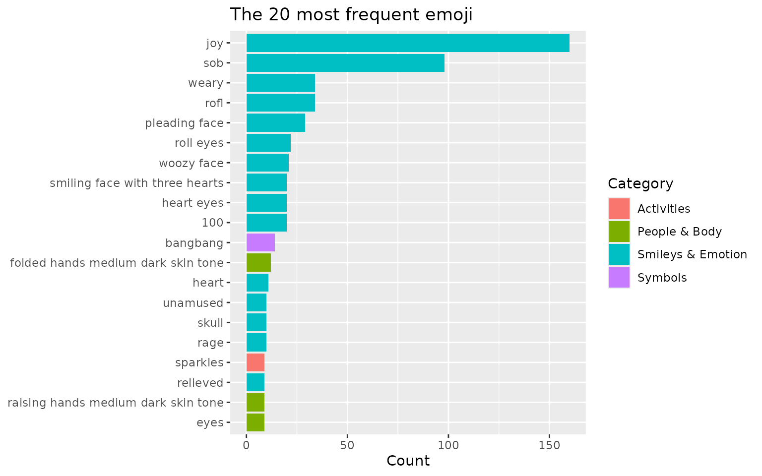

The unicode column holds the actual glyph, should you wish to render the emoji themselves on a plot (this requires a graphics device with an emoji-capable font). You can also request a different number of emoji:

ata_tweets %>%
  top_n_emojis(full_text, n = 10) %>%
  mutate(emoji_name = stringr::str_replace_all(emoji_name, "_", " "),
         emoji_name = forcats::fct_reorder(emoji_name, n)) %>%
  ggplot(aes(n, emoji_name, fill = emoji_category)) +
  geom_col() +
  labs(x = "Count", y = NULL, fill = "Category",
       title = "The 10 most frequent emoji")

Categorising emoji

The Unicode standard organises emoji into 10 categories (see ?category_unicode_crosswalk). emoji_categorize() keeps the emoji-bearing rows and adds a .emoji_category column listing the distinct categories present in each row, separated by | when a row spans more than one.

ata_emoji_category <- ata_tweets %>%
  emoji_categorize(full_text) %>%
  select(.emoji_category)

ata_emoji_category
#> # A tibble: 560 × 1
#>    .emoji_category  
#>    <chr>            
#>  1 Smileys & Emotion
#>  2 Smileys & Emotion
#>  3 Smileys & Emotion
#>  4 Smileys & Emotion
#>  5 Smileys & Emotion
#>  6 People & Body    
#>  7 Smileys & Emotion
#>  8 Smileys & Emotion
#>  9 Smileys & Emotion
#> 10 Smileys & Emotion
#> # ℹ 550 more rows

We can tally the most common category combinations:

ata_emoji_category %>%
  count(.emoji_category, sort = TRUE) %>%
  filter(n > 20) %>%
  mutate(.emoji_category = forcats::fct_reorder(.emoji_category, n)) %>%
  ggplot(aes(n, .emoji_category)) +
  geom_col() +
  labs(x = "Number of entries", y = NULL,
       title = "Most common emoji category combinations")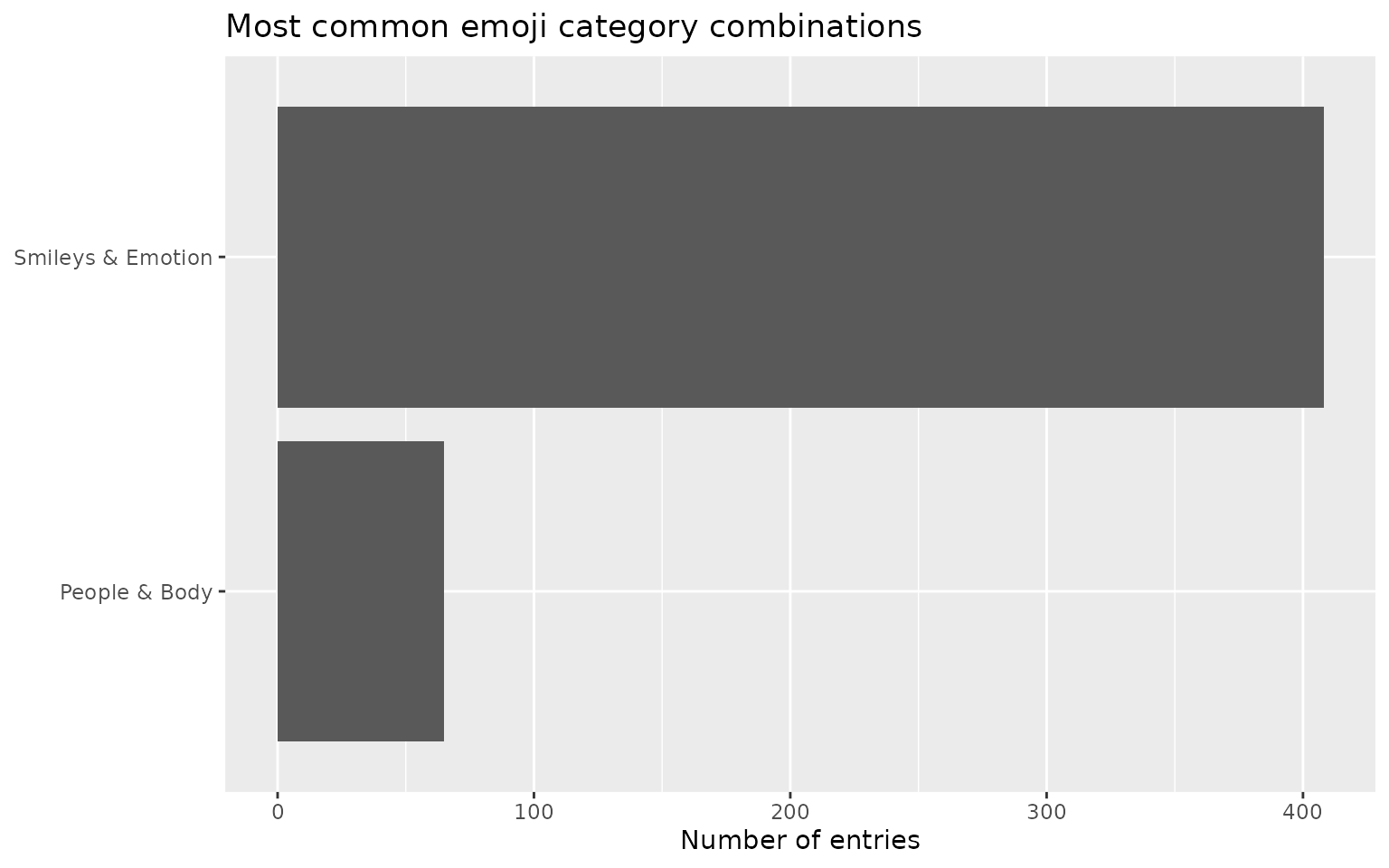

To count the 10 individual categories rather than their combinations, split the .emoji_category strings on | with tidyr::separate_rows():

ata_emoji_category %>%
  tidyr::separate_rows(.emoji_category, sep = "\\|") %>%
  count(.emoji_category, sort = TRUE) %>%
  mutate(.emoji_category = forcats::fct_reorder(.emoji_category, n)) %>%
  ggplot(aes(n, .emoji_category)) +
  geom_col() +
  labs(x = "Number of entries", y = NULL,
       title = "Emoji category usage")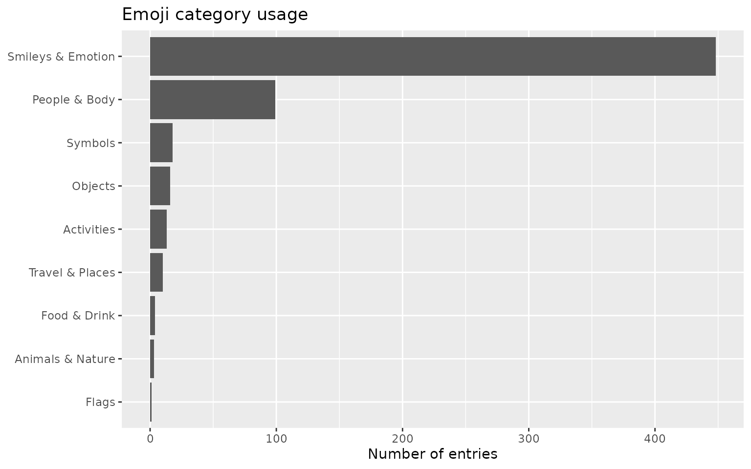

“Smileys & Emotion” dominates, followed by “People & Body”. Note that an entry spanning several categories is counted once in each, so these counts can exceed the number of emoji-bearing entries.

emoji_type(): faces versus everything else

The consumer-behaviour literature repeatedly contrasts emotional (face) emoji with semantic (object) emoji and finds that the two have different effects on engagement. emoji_type() recodes the Unicode group and subgroup into that smaller functional vocabulary, and emoji_faceness() reduces it to a single per-entry share:

ata_tweets %>%
  emoji_type(full_text) %>%
  count(.emoji_type, sort = TRUE) %>%
  head(5)
#> # A tibble: 5 × 2
#>   .emoji_type     n
#>   <chr>       <int>
#> 1 NA           1440
#> 2 face          364
#> 3 gesture        54
#> 4 symbol         42
#> 5 face|symbol    17

ata_tweets %>%
  emoji_faceness(full_text) %>%
  summarise(mean_faceness = mean(.emoji_faceness, na.rm = TRUE),
            all_faces = sum(.emoji_faceness == 1, na.rm = TRUE))
#> # A tibble: 1 × 2
#>   mean_faceness all_faces
#>           <dbl>     <int>
#> 1         0.694       364

as_emoji_type() is the vector-level version, for typing a glyph you already have in hand.

Scoring emoji sentiment

emoji_sentiment()

Emoji are a strong sentiment signal, and emoji_sentiment() surfaces it directly. It adds .emoji_n (the number of emoji in the entry), .emoji_n_scored (the number that appear in the lexicon), and .emoji_sentiment (the mean sentiment of the scored emoji, from -1 to +1). Scores come from the bundled emoji_sentiment_lexicon (described below); entries with no emoji, or whose emoji are not in the lexicon, receive NA.

ata_sentiment <- ata_tweets %>%
  emoji_sentiment(full_text)

ata_sentiment %>%
  select(.emoji_n, .emoji_sentiment)
#> # A tibble: 2,000 × 2
#>    .emoji_n .emoji_sentiment
#>       <int>            <dbl>
#>  1        0          NA     
#>  2        1          -0.0934
#>  3        0          NA     
#>  4        1          -0.0934
#>  5        0          NA     
#>  6        0          NA     
#>  7        0          NA     
#>  8        0          NA     
#>  9        0          NA     
#> 10        1          NA     
#> # ℹ 1,990 more rows

Sentiment distribution

Looking across the entries that contain at least one scored emoji:

ata_sentiment %>%
  filter(!is.na(.emoji_sentiment)) %>%
  ggplot(aes(.emoji_sentiment)) +
  geom_histogram(binwidth = 0.1) +
  labs(x = "Mean emoji sentiment",
       y = "Number of entries",
       title = "Emoji sentiment skews positive")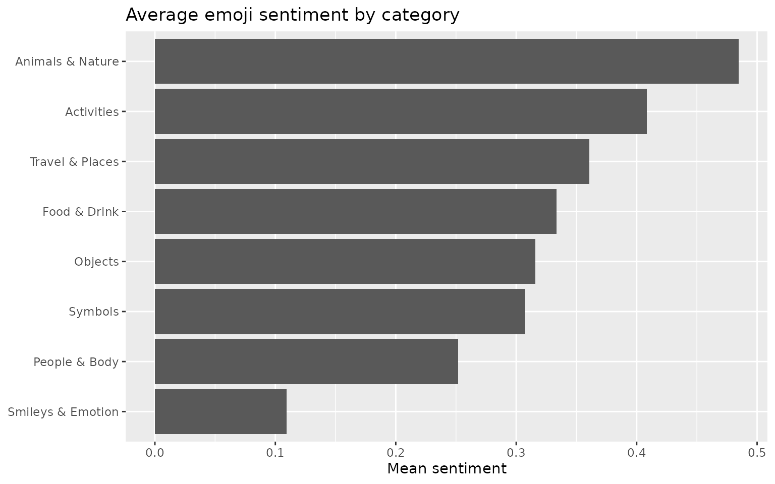

As is typical of social-media text, emoji sentiment leans strongly positive.

Sentiment by category

Because emoji_tokens() attaches a sentiment score to every emoji occurrence, we can summarise average sentiment by category in a couple of lines:

ata_tweets %>%
  emoji_tokens(full_text) %>%
  group_by(.emoji_category) %>%
  summarise(mean_sentiment = mean(.emoji_sentiment, na.rm = TRUE),
            n_scored = sum(!is.na(.emoji_sentiment))) %>%
  filter(n_scored > 0) %>%
  mutate(.emoji_category = forcats::fct_reorder(.emoji_category, mean_sentiment)) %>%
  ggplot(aes(mean_sentiment, .emoji_category)) +
  geom_col() +
  labs(x = "Mean sentiment", y = NULL,
       title = "Average emoji sentiment by category")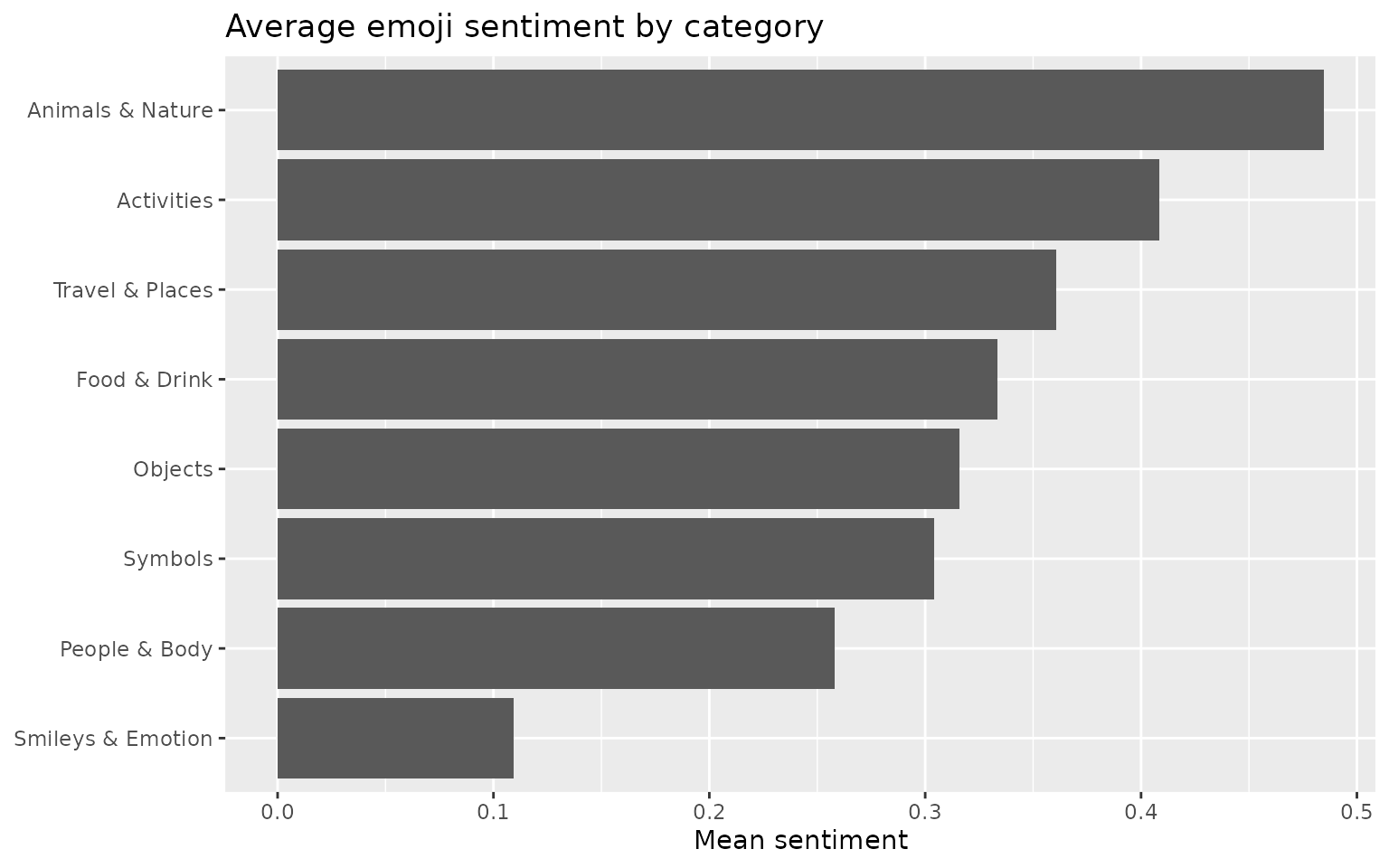

The sentiment lexicon

The scores come from emoji_sentiment_lexicon, the Emoji Sentiment Ranking of Kralj Novak et al. (2015), computed from around 70,000 tweets annotated in 13 European languages. You can work with it directly — for instance, to find the most positive and most negative reasonably common emoji:

emoji_sentiment_lexicon %>%
  filter(occurrences >= 500) %>%
  slice_max(sentiment_score, n = 8) %>%
  select(emoji, unicode_name, occurrences, sentiment_score)
#>   emoji         unicode_name occurrences sentiment_score
#> 1     ❤    HEAVY BLACK HEART        8050       0.7460870
#> 2    💞     REVOLVING HEARTS         687       0.7423581
#> 3    🎉         PARTY POPPER        1125       0.7395556
#> 4    💃               DANCER        1344       0.7358631
#> 5    💙           BLUE HEART         912       0.7324561
#> 6    💖      SPARKLING HEART        1263       0.7133808
#> 7    💛         YELLOW HEART         602       0.7126246
#> 8    😘 FACE THROWING A KISS        3648       0.7017544

emoji_sentiment_lexicon %>%
  filter(occurrences >= 500) %>%
  slice_min(sentiment_score, n = 8) %>%
  select(emoji, unicode_name, occurrences, sentiment_score)
#>   emoji       unicode_name occurrences sentiment_score
#> 1    😒      UNAMUSED FACE        1385     -0.37472924
#> 2    😩         WEARY FACE        1808     -0.36836283
#> 3    🔫             PISTOL         604     -0.19536424
#> 4    😡       POUTING FACE         756     -0.17328042
#> 5    😔       PENSIVE FACE        1205     -0.14605809
#> 6    😞  DISAPPOINTED FACE         532     -0.11842105
#> 7    😭 LOUDLY CRYING FACE        5526     -0.09337676
#> 8    😴      SLEEPING FACE         718     -0.08077994

Interpretation risk: how much do readers disagree?

The most practically important fact about emoji is that people do not agree on what they mean. Miller et al. (2016) showed the same rendering to many readers and found they disagreed about whether it was positive, neutral or negative around a quarter of the time.

That disagreement was already inside the package. The Emoji Sentiment Ranking keeps the raw negative/neutral/positive annotation counts behind its collapsed score, which is an empirical interpretation distribution per glyph. emoji_ambiguity() reads it out:

emoji_ambiguity() %>%
  filter(n_annotations > 500) %>%
  head(5)
#> # A tibble: 5 × 8
#>   emoji key   n_annotations p_neg p_neu p_pos ambiguity  rank
#>   <chr> <chr>         <int> <dbl> <dbl> <dbl>     <dbl> <int>
#> 1 😳    1F633           846 0.327 0.327 0.345      1.10     6
#> 2 💯    1F4AF           637 0.281 0.317 0.402      1.09    16
#> 3 😴    1F634           718 0.422 0.237 0.341      1.07    43
#> 4 😢    1F622           749 0.385 0.224 0.391      1.07    47
#> 5 😱    1F631          1130 0.264 0.282 0.454      1.07    50

Because the measure is a property of the glyph, the corpus-level question – “which of my emoji are most likely to be misread?” – is one call:

ata_tweets %>%
  emoji_flag_ambiguous(full_text, top_n = 5)
#> # A tibble: 5 × 6
#>   emoji name               n n_annotations ambiguity  rank
#>   <chr> <chr>          <int>         <int>     <dbl> <int>
#> 1 😳    flushed face       3           846      1.10     6
#> 2 💣    bomb               2           131      1.09    10
#> 3 💯    hundred points    20           637      1.09    16
#> 4 😯    hushed face        1            62      1.08    20
#> 5 💔    broken heart       5           328      1.08    22

emoji_risk() is the per-entry version, and the pair .emoji_n / .emoji_n_scored keeps the coverage honest: an entry whose emoji are absent from the lexicon is not a low-risk entry, it is an unmeasured one.

ata_tweets %>%
  emoji_risk(full_text) %>%
  filter(.emoji_n > 1) %>%
  select(.emoji_n, .emoji_n_scored, .emoji_ambiguity_mean,
         .emoji_n_ambiguous) %>%
  head(5)
#> # A tibble: 5 × 4
#>   .emoji_n .emoji_n_scored .emoji_ambiguity_mean .emoji_n_ambiguous
#>      <int>           <int>                 <dbl>              <int>
#> 1        2               2                 1.06                   2
#> 2        2               2                 1.06                   2
#> 3        2               2                 0.973                  1
#> 4        2               2                 1.06                   2
#> 5        3               2                 0.889                  1

The same counts also put an error bar on the sentiment score itself. A glyph annotated eight times should not carry the authority of one annotated eight thousand times, and emoji_sentiment(se = TRUE) says so:

ata_tweets %>%
  emoji_sentiment(full_text, se = TRUE) %>%
  filter(!is.na(.emoji_sentiment)) %>%
  select(.emoji_n_scored, .emoji_sentiment, .emoji_sentiment_se) %>%
  head(5)
#> # A tibble: 5 × 3
#>   .emoji_n_scored .emoji_sentiment .emoji_sentiment_se
#>             <int>            <dbl>               <dbl>
#> 1               1          -0.0934             0.0118 
#> 2               1          -0.0934             0.0118 
#> 3               1           0.221              0.00675
#> 4               1           0.746              0.00587
#> 5               1          -0.0934             0.0118

Scoring emoji emotions

Valence (negative↔︎positive) is only one affective dimension. emoji_emotion() goes further, scoring each entry’s emoji across the eight Plutchik emotions (anger, anticipation, disgust, fear, joy, sadness, surprise, trust) using the bundled EmoTag1200 lexicon (Shoeb & de Melo, 2020). Scores are in [0, 1].

ata_emotion <- ata_tweets %>%
  emoji_emotion(full_text)

ata_emotion %>%
  select(.emoji_joy, .emoji_trust, .emoji_anger, .emoji_n)
#> # A tibble: 2,000 × 4
#>    .emoji_joy .emoji_trust .emoji_anger .emoji_n
#>         <dbl>        <dbl>        <dbl>    <int>
#>  1         NA        NA           NA           0
#>  2          0         0.08         0.22        1
#>  3         NA        NA           NA           0
#>  4          0         0.08         0.22        1
#>  5         NA        NA           NA           0
#>  6         NA        NA           NA           0
#>  7         NA        NA           NA           0
#>  8         NA        NA           NA           0
#>  9         NA        NA           NA           0
#> 10         NA        NA           NA           1
#> # ℹ 1,990 more rows

A quick way to read the result is the dominant emotion per entry:

ata_tweets %>%
  emoji_emotion_label(full_text) %>%
  count(.emoji_emotion, sort = TRUE)
#> # A tibble: 9 × 2
#>   .emoji_emotion     n
#>   <chr>          <int>
#> 1 NA              1639
#> 2 joy              166
#> 3 sadness          115
#> 4 anticipation      30
#> 5 surprise          15
#> 6 anger             12
#> 7 disgust           11
#> 8 fear              10
#> 9 trust              2

The emotion scores join through the same codepoint-normalised key as sentiment, so emoji carrying the U+FE0F variation selector resolve correctly.

Bringing your own lexicon

Sentiment and emotion scoring share one pluggable engine. emoji_lexicons() lists the bundled lexicons (plus any you have registered):

emoji_lexicons()
#> # A tibble: 2 × 6
#>   name       type      dimensions     n source                           licence
#>   <chr>      <chr>     <I<list>>  <int> <chr>                            <chr>  
#> 1 novak2015  sentiment <chr [1]>    969 Kralj Novak et al. (2015), PLoS… CC BY-…
#> 2 emotag1200 emotion   <chr [8]>    150 Shoeb & de Melo (2020), EMNLP 2… MIT

emoji_score() is the generic scorer underneath emoji_sentiment(): give it any data frame with an emoji column and a score column — say, scores tailored to your own domain — and it returns the per-row mean, joined through the same codepoint-normalised key as everything else:

my_lexicon <- data.frame(
  emoji = c("\U0001f600", "\U0001f621", "\U0001f637"),
  score = c(1, -1, -0.5)
)

data.frame(text = c("great \U0001f600", "bad \U0001f621\U0001f637", "none")) %>%
  emoji_score(text, lexicon = my_lexicon)
#> # A tibble: 3 × 4
#>   text     .emoji_score .emoji_n_scored .emoji_n
#>   <chr>           <dbl>           <int>    <int>
#> 1 great 😀         1                  1        1
#> 2 bad 😡😷        -0.75               2        2
#> 3 none            NA                 NA        0

register_emoji_lexicon() stores a lexicon under a name for the session, so you can refer to it in emoji_score() — or in emoji_emotion(), if it carries emotion columns:

register_emoji_lexicon("mine", my_lexicon)
emoji_lexicons() %>% filter(name == "mine")
#> # A tibble: 1 × 6
#>   name  type   dimensions     n source          licence
#>   <chr> <chr>  <I<list>>  <int> <chr>           <chr>  
#> 1 mine  custom <chr [1]>      3 user-registered NA

Relating emoji: co-occurrence and sequences

Which emoji appear together? emoji_pairs() returns a tidy edge list — one row per pair of distinct emoji that co-occur in the same entry, with the number of entries in which they do. The item1/item2/n shape matches widyr::pairwise_count() and feeds directly into graph tools such as igraph, tidygraph and ggraph:

emoji_edges <- ata_tweets %>%
  emoji_pairs(full_text)

emoji_edges
#> # A tibble: 213 × 3
#>    item1 item2     n
#>    <chr> <chr> <int>
#>  1 😂    😭       10
#>  2 😂    😩        4
#>  3 😂    🙄        3
#>  4 😭    🙄        3
#>  5 💕    🥰        2
#>  6 💞    🥺        2
#>  7 💯    🤷🏽‍♂️        2
#>  8 😂    🤔        2
#>  9 😂    🤣        2
#> 10 😂    🤷🏼‍♀️        2
#> # ℹ 203 more rows

The strongest pairings make a readable chart on their own:

emoji_edges %>%
  slice_max(n, n = 10) %>%
  mutate(pair = paste(item1, item2),
         pair = forcats::fct_reorder(pair, n)) %>%
  ggplot(aes(n, pair)) +
  geom_col() +
  labs(x = "Number of entries containing both", y = NULL,
       title = "Emoji that appear together")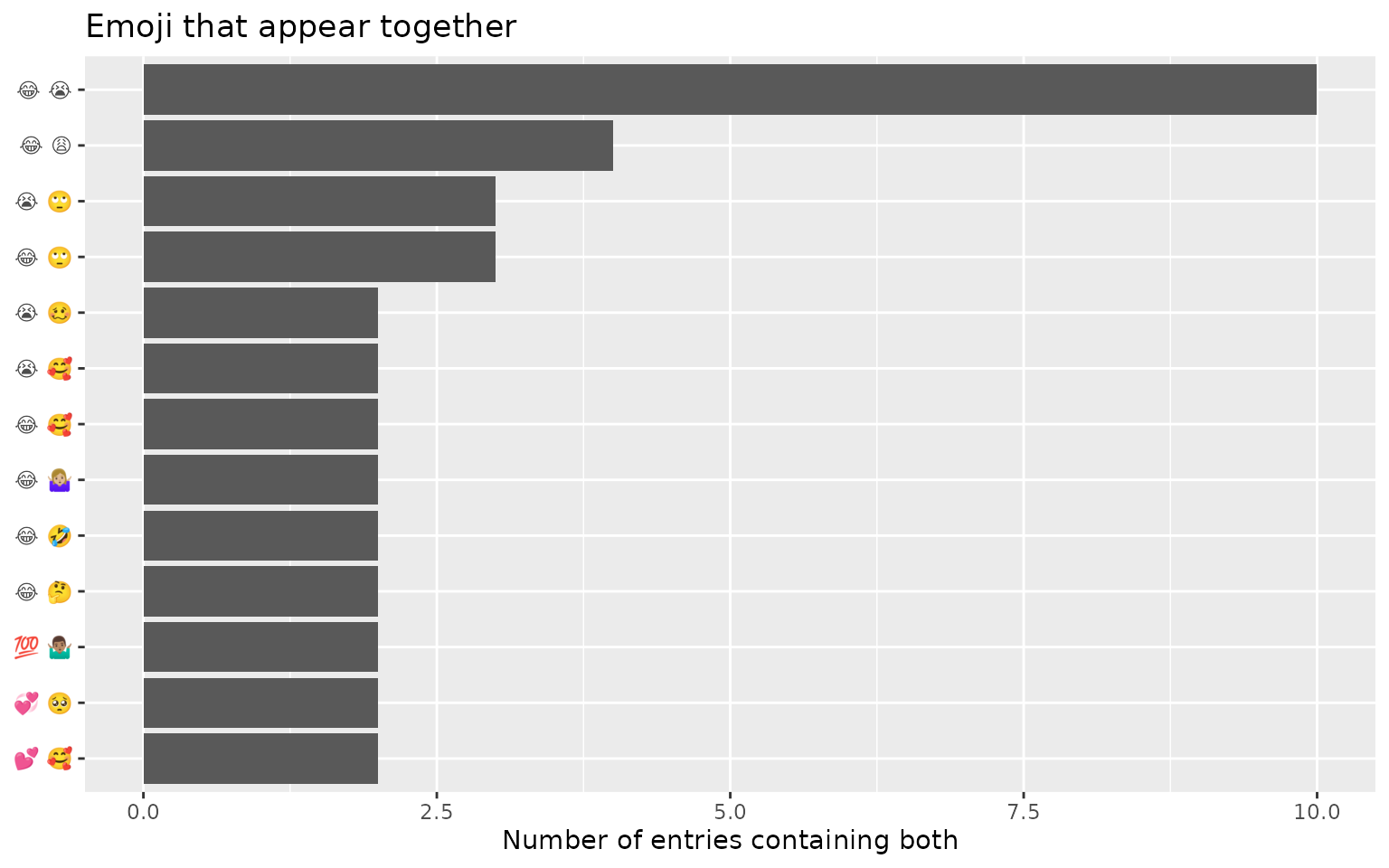

Set directed = TRUE to order each pair by first appearance, or supply doc_id to pool several rows (a conversation, a user, a day) into one document. emoji_cooccurrence(diagonal = TRUE) additionally returns each emoji’s document frequency on the diagonal.

Order also matters within an entry. emoji_ngrams() slides a window over each entry’s emoji in reading order (any text in between is ignored), which is the raw material for sequence and Markov-style analyses:

ata_tweets %>%
  emoji_ngrams(full_text) %>%
  count(.emoji_ngram, sort = TRUE)
#> # A tibble: 158 × 2
#>    .emoji_ngram     n
#>    <chr>        <int>
#>  1 😂 😂           66
#>  2 😭 😭           27
#>  3 😍 😍           13
#>  4 🥺 🥺           13
#>  5 🤣 🤣           10
#>  6 😭 😂            8
#>  7 🖕🏻 🖕🏻            7
#>  8 😡 😡            5
#>  9 🙏🏾 🙏🏾            5
#> 10 💀 💀            4
#> # ℹ 148 more rows

All the relational verbs canonicalise glyphs through the same codepoint-normalised key as the rest of the package, so qualified and unqualified forms of one emoji count as a single node.

The words around an emoji

Which emoji occurred is only half the story: emoji are polysemous, and their reading is decided by the co-text. emoji_context() returns one row per occurrence with a window of the surrounding text. Other emoji are blanked out of the window, so a neighbouring glyph never leaks into it:

ata_tweets %>%
  emoji_context(full_text, window = 4) %>%
  select(.row_number, .emoji, .emoji_context) %>%
  head(5)
#> # A tibble: 5 × 3
#>   .row_number .emoji .emoji_context                   
#>         <int> <chr>  <chr>                            
#> 1           2 😭     stuck here in Brunswick          
#> 2           4 😭     fever nonstop by Wizkid          
#> 3          10 🙄     Phone dry asf                    
#> 4          15 😂     lot of white girls . I thought it
#> 5          17 ❤️      needs self care days

Aggregated over a corpus, those windows give the emoji-word associations that a sense inventory would otherwise have to supply – derived from your own data, so they are neither stale nor licence-encumbered:

ata_tweets %>%
  emoji_collocations(full_text, window = 4, min_n = 5) %>%
  head(10)
#> # A tibble: 10 × 4
#>    emoji word          n   pmi
#>    <chr> <chr>     <int> <dbl>
#>  1 🙌🏾    god           5  4.31
#>  2 🖕🏻    underdogs     8  3.93
#>  3 😍    lacking      11  3.49
#>  4 😍    strapped     11  3.49
#>  5 😍    yess         11  3.49
#>  6 🥺    everytime     7  3.44
#>  7 🥺    greys         7  3.44
#>  8 🥺    accepted      5  3.44
#>  9 🥺    clemson       5  3.44
#> 10 🥺    into          5  3.44

Tokenisation stops at whitespace on purpose. If you need stemming or stopword removal, hand the result to tidytext rather than expecting this verb to grow a tokeniser.

Measuring how emoji are used

Where emoji sit and how much of the text they occupy are studied signals in their own right. emoji_position() reports each entry’s first and last emoji position and the mean relative position from 0 (start) to 1 (end):

ata_tweets %>%
  emoji_position(full_text) %>%
  filter(!is.na(.emoji_rel_position)) %>%
  ggplot(aes(.emoji_rel_position)) +
  geom_histogram(binwidth = 0.05) +
  labs(x = "Mean relative position of the entry's emoji",
       y = "Number of entries",
       title = "Emoji cluster at the end of a message")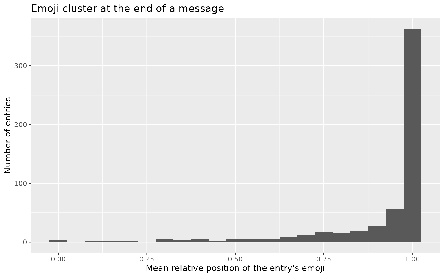

emoji_density() normalises the emoji count by text length (per character and per whitespace-delimited token), and emoji_ratio() reports what share of the text’s characters belong to emoji — including an .emoji_only flag for entries that are nothing but emoji (and whitespace):

ata_tweets %>%
  emoji_ratio(full_text) %>%
  summarise(
    n_emoji_only = sum(.emoji_only, na.rm = TRUE),
    mean_ratio   = mean(.emoji_ratio[.emoji_ratio > 0], na.rm = TRUE)
  )
#> # A tibble: 1 × 2
#>   n_emoji_only mean_ratio
#>          <int>      <dbl>
#> 1            0     0.0405

Emoji over time

Almost every substantive emoji study is longitudinal. Our sample has no timestamp, so the dates below are synthetic – they illustrate the mechanics, not a finding:

dated <- ata_tweets %>%
  mutate(posted_at = as.Date("2021-01-01") + (seq_len(n()) - 1) %% 540)

dated %>%
  emoji_trend(full_text, posted_at, by = "quarter", top_n = 3)
#> # A tibble: 18 × 5
#>    .period    emoji name                       n   share
#>    <date>     <chr> <chr>                  <int>   <dbl>
#>  1 2021-01-01 😂    face with tears of joy    31 0.194  
#>  2 2021-01-01 😭    loudly crying face        17 0.106  
#>  3 2021-01-01 😩    weary face                 9 0.0562 
#>  4 2021-04-01 😂    face with tears of joy    42 0.214  
#>  5 2021-04-01 😩    weary face                 8 0.0408 
#>  6 2021-04-01 😭    loudly crying face         8 0.0408 
#>  7 2021-07-01 😭    loudly crying face        26 0.166  
#>  8 2021-07-01 😂    face with tears of joy    22 0.140  
#>  9 2021-07-01 😩    weary face                 3 0.0191 
#> 10 2021-10-01 😂    face with tears of joy    34 0.221  
#> 11 2021-10-01 😭    loudly crying face        13 0.0844 
#> 12 2021-10-01 😩    weary face                 9 0.0584 
#> 13 2022-01-01 😂    face with tears of joy    18 0.157  
#> 14 2022-01-01 😭    loudly crying face        12 0.104  
#> 15 2022-01-01 😩    weary face                 4 0.0348 
#> 16 2022-04-01 😭    loudly crying face        22 0.186  
#> 17 2022-04-01 😂    face with tears of joy    13 0.110  
#> 18 2022-04-01 😩    weary face                 1 0.00847

emoji_turnover() asks a different question – not how often an emoji is used but how much of the repertoire changes from one period to the next:

dated %>%
  emoji_turnover(full_text, posted_at, by = "quarter")
#> # A tibble: 5 × 8
#>   .period    .period_prev n_types_prev n_types jaccard n_new n_lost n_core
#>   <date>     <date>              <int>   <int>   <dbl> <int>  <int>  <int>
#> 1 2021-04-01 2021-01-01             56      79   0.298    48     25     31
#> 2 2021-07-01 2021-04-01             79      57   0.225    32     54     25
#> 3 2021-10-01 2021-07-01             57      65   0.232    42     34     23
#> 4 2022-01-01 2021-10-01             65      56   0.260    31     40     25
#> 5 2022-04-01 2022-01-01             56      49   0.25     28     35     21

Two of the time verbs need no timestamp at all, because the reference table already records the Unicode version that introduced each glyph. That makes “how new is this corpus’s emoji vocabulary?” a single call:

ata_tweets %>%
  emoji_version_profile(full_text) %>%
  head(8)
#> # A tibble: 8 × 7
#>   version version_num release_date n_types n_tokens share_types share_tokens
#>   <chr>         <dbl> <date>         <int>    <int>       <dbl>        <dbl>
#> 1 0.6             0.6 2010-10-11        74      517     0.396        0.574  
#> 2 0.7             0.7 2014-06-16         1        4     0.00535      0.00444
#> 3 1.0             1   2015-06-09        44      126     0.235        0.14   
#> 4 2.0             2   2015-11-12         1        1     0.00535      0.00111
#> 5 3.0             3   2016-06-21        17       58     0.0909       0.0644 
#> 6 4.0             4   2016-11-22        17       38     0.0909       0.0422 
#> 7 5.0             5   2017-06-20         8       19     0.0428       0.0211 
#> 8 11.0           11   2018-06-05         8       84     0.0428       0.0933

With real timestamps, emoji_adoption_lag() goes one step further and compares each glyph’s first appearance in the corpus with its Unicode release date – see emoji_unicode_releases() for that lookup, and emoji_seasonality() for month-of-year, day-of-week and hour-of-day cycles.

Emoji as model features

For classification and regression work, emoji_dfm() turns the corpus into a document-by-emoji feature table: one row per entry (or per doc_id), one column per emoji, weighted by counts, binary presence or tf-idf. Every entry is kept — emoji-free rows are all zeros — so the table binds row-for-row to your outcome columns:

ata_tweets %>%
  emoji_dfm(full_text, weighting = "tfidf") %>%
  select(1:6)
#> # A tibble: 2,000 × 6
#>    .row_number  `😂`  `😭`  `😩`  `🤣`  `🥺`
#>          <int> <dbl> <dbl> <dbl> <dbl> <dbl>
#>  1           1     0  0        0     0     0
#>  2           2     0  3.34     0     0     0
#>  3           3     0  0        0     0     0
#>  4           4     0  3.34     0     0     0
#>  5           5     0  0        0     0     0
#>  6           6     0  0        0     0     0
#>  7           7     0  0        0     0     0
#>  8           8     0  0        0     0     0
#>  9           9     0  0        0     0     0
#> 10          10     0  0        0     0     0
#> # ℹ 1,990 more rows

Text-emoji mismatch

Two separate literatures converge on one statistic. NLP sarcasm detection uses emoji-text sentiment incongruity as a feature; marketing research finds that a mismatch between a review’s words and its emoji lowers perceived helpfulness and authenticity. Both want the same number.

tidyEmoji deliberately does not score text – that choice belongs in your script, where the method is visible. Here is a deliberately crude word-list scorer standing in for tidytext + AFINN, sentimentr or a transformer:

positive <- c("love", "great", "best", "happy", "good", "thanks", "beautiful")
negative <- c("hate", "worst", "bad", "sad", "awful", "sick", "tired")

scored <- ata_tweets %>%
  mutate(text_score = vapply(
    strsplit(tolower(full_text), "[^a-z]+"),
    function(w) as.numeric(sum(w %in% positive) - sum(w %in% negative)),
    numeric(1)
  ))

scale has no default: AFINN runs -5 to 5, VADER -1 to 1, and a model’s logits on nothing in particular, so you have to say how the two sides were made comparable. "rank" puts both on percentiles and is the safest choice.

incong <- scored %>%
  emoji_incongruity(full_text, text_score, scale = "rank")

incong %>%
  filter(!is.na(.emoji_incongruity)) %>%
  count(.emoji_polarity_flip)
#> # A tibble: 2 × 2
#>   .emoji_polarity_flip     n
#>   <lgl>                <int>
#> 1 FALSE                  358
#> 2 TRUE                    15

incong %>%
  filter(.emoji_polarity_flip) %>%
  select(full_text, .emoji_sentiment, text_score) %>%
  head(3)
#> # A tibble: 3 × 3
#>   full_text                                          .emoji_sentiment text_score
#>   <chr>                                                         <dbl>      <dbl>
#> 1 zay hilfiger went from juju on that BEAT , to juj…           0.0245         -1
#> 2 Worst story 📖 I heard. I guy I met bought 200 sha…           0.176          -1
#> 3 Ew don’t you hate when a hoe watch you and you do…           0.221          -1

Note what happens to entries with no scorable emoji: they get NA, never 0. A neutral emoji and no emoji at all are different states, and collapsing them biases every model downstream. emoji_incongruity_profile() aggregates the same numbers by glyph, and emoji_congruence() is the identical engine under the marketing framing.

scored %>%
  emoji_incongruity_profile(full_text, text_score, scale = "rank", min_n = 10)
#> # A tibble: 9 × 7
#>   emoji name                 n mean_incongruity sd_incongruity n_flips flip_rate
#>   <chr> <chr>            <int>            <dbl>          <dbl>   <int>     <dbl>
#> 1 😂    face with tears…   160           0.233         0.382         9    0.0562
#> 2 😭    loudly crying f…    98          -0.265         0.400         3    0.0306
#> 3 😩    weary face          34          -0.587         0.476         1    0.0294
#> 4 💯    hundred points      20           0.0123        0.278         0    0     
#> 5 😍    smiling face wi…    20           0.876         0.223         0    0     
#> 6 ❤️     red heart           11           0.967         0.129         0    0     
#> 7 💀    skull               10          -0.620         0.255         0    0     
#> 8 😒    unamused face       10          -0.892         0.00850       0    0     
#> 9 😡    enraged face        10          -0.447         0.320         0    0

Translating emoji to and from text

Replacing emoji with words is useful for accessibility (screen readers) and as an NLP normalisation step before tokenising. emoji_to_text() does this for a whole column, in either Unicode-name or shortcode form; text_to_emoji() is the inverse.

demo <- data.frame(text = "great \U0001f600 love \u2764\ufe0f")
demo %>% emoji_to_text(text, format = "name")
#> # A tibble: 1 × 1
#>   text                              
#>   <chr>                             
#> 1 great grinning face love red heart
demo %>% emoji_to_text(text, format = "shortcode")
#> # A tibble: 1 × 1
#>   text                         
#>   <chr>                        
#> 1 great :grinning: love :heart:
demo %>%
  emoji_to_text(text, format = "shortcode") %>%
  text_to_emoji(text)
#> # A tibble: 1 × 1
#>   text           
#>   <chr>          
#> 1 great 😀 love ❤️

Note that the qualified heart (which carries the U+FE0F variation selector) translates just as reliably as any other emoji, thanks to the normalised join key. For ad-hoc, vector-level use there are also as_emoji_name(), as_emoji_shortcode() and as_emoji():

as_emoji_name(c("\U0001f600", "\u2764\ufe0f"))
#> [1] "grinning face" "red heart"
as_emoji_shortcode(c("\U0001f600", "\u2764\ufe0f"))
#> [1] "grinning" "heart"
as_emoji(c("grinning", "heart"))
#> [1] "😀" "❤️"

Searching the emoji catalogue

emoji_search() looks emoji up by keyword, name or shortcode (case-insensitive, literal matching), returning a tidy tibble you can filter further or feed into the other verbs:

emoji_search("happy")
#> # A tibble: 27 × 5
#>    emoji name                            shortcode             group     keyword
#>    <chr> <chr>                           <chr>                 <chr>     <chr>  
#>  1 😀    grinning face                   grinning              Smileys … happy  
#>  2 😃    grinning face with big eyes     smiley                Smileys … happy  
#>  3 😄    grinning face with smiling eyes smile                 Smileys … happy  
#>  4 😁    beaming face with smiling eyes  grin                  Smileys … happy  
#>  5 😆    grinning squinting face         laughing              Smileys … happy  
#>  6 🤣    rolling on the floor laughing   rofl                  Smileys … happy  
#>  7 😂    face with tears of joy          joy                   Smileys … happy  
#>  8 🙂    slightly smiling face           slightly_smiling_face Smileys … happy  
#>  9 😇    smiling face with halo          innocent              Smileys … happy  
#> 10 ☺     smiling face                    smiling_face          Smileys … happy  
#> # ℹ 17 more rows
emoji_search("celebration")
#> # A tibble: 27 × 5
#>    emoji name                     shortcode      group             keyword    
#>    <chr> <chr>                    <chr>          <chr>             <chr>      
#>  1 🥳    partying face            partying_face  Smileys & Emotion celebration
#>  2 🙌    raising hands            raised_hands   People & Body     celebration
#>  3 🎅    Santa Claus              santa          People & Body     celebration
#>  4 🤶    Mrs. Claus               mrs_claus      People & Body     celebration
#>  5 🧑‍🎄    Mx Claus                 mx_claus       People & Body     celebration
#>  6 🎂    birthday cake            birthday       Food & Drink      celebration
#>  7 🍾    bottle with popping cork champagne      Food & Drink      celebration
#>  8 🎃    jack-o-lantern           jack_o_lantern Activities        celebration
#>  9 🎄    Christmas tree           christmas_tree Activities        celebration
#> 10 🎆    fireworks                fireworks      Activities        celebration
#> # ℹ 17 more rows

Emoji in language-model pipelines

Emoji are now a preprocessing decision in every LLM pipeline, and the decision matters: they inflate token counts several-fold, and models disambiguate them poorly. emoji_token_cost() gives the exact sizes plus a clearly-labelled estimate – pass your real tokeniser through tokenizer when the number matters:

ata_tweets %>%
  emoji_token_cost(full_text) %>%
  filter(.emoji_n > 0) %>%
  summarise(emoji = sum(.emoji_n),
            bytes = sum(.emoji_bytes),
            codepoints = sum(.emoji_codepoints),
            est_tokens = sum(.emoji_token_estimate))
#> # A tibble: 1 × 4
#>   emoji bytes codepoints est_tokens
#>   <int> <int>      <int>      <int>
#> 1   900  4437       1166       2245

emoji_sanitize() then applies one named policy to the column. The capability is not new – most of it exists across emoji_to_text() and the extraction verbs – but the named argument shows up in a script diff and in a methods section, which is the point:

demo_llm <- data.frame(text = "ship it \U0001f680 today")
for (p in c("keep", "strip", "name", "shortcode", "placeholder")) {
  cat(format(p, width = 12), emoji_sanitize(demo_llm, text, policy = p)$text,
      "\n")
}
#> keep         ship it 🚀 today 
#> strip        ship it today 
#> name         ship it rocket today 
#> shortcode    ship it :rocket: today 
#> placeholder  ship it [emoji] today

Recording provenance

“Emoji” is not a fixed object. Which glyphs exist, what they are called and which lexicon scored them all depend on versions, and a result is not reproducible without them. emoji_provenance() puts the lot in one row you can paste into a methods section:

emoji_provenance() %>% glimpse()
#> Rows: 1
#> Columns: 7
#> $ tidyEmoji         <chr> "0.4.0"
#> $ emoji_pkg         <chr> "16.0.0"
#> $ unicode_emoji     <chr> "16.0"
#> $ n_emoji           <int> 5042
#> $ sentiment_lexicon <chr> "novak2015 (969 emoji)"
#> $ emotion_lexicon   <chr> "emotag1200 (150 emoji)"
#> $ R                 <chr> "4.6.1"

Bundled datasets

tidyEmoji ships four datasets, each documented with its own help page:

• emoji_sentiment_lexicon — emoji sentiment scores from the Emoji Sentiment Ranking (see ?emoji_sentiment_lexicon).
• emoji_emotion_lexicon — emoji emotion scores from EmoTag1200 (see ?emoji_emotion_lexicon).
• emoji_unicode_crosswalk — one row per emoji name, mapping names / shortcodes to glyphs and categories.
• category_unicode_crosswalk — one row per Unicode category, listing its emoji.

These are regenerated from the current Unicode emoji list by the scripts in the package’s data-raw/ directory.

References

Kralj Novak P, Smailović J, Sluban B, Mozetič I (2015). Sentiment of Emojis. PLoS ONE 10(12): e0144296. https://doi.org/10.1371/journal.pone.0144296. The Emoji Sentiment Ranking is distributed under the Creative Commons Attribution-ShareAlike 4.0 International (CC BY-SA 4.0) licence.

Miller H, Thebault-Spieker J, Chang S, Johnson I, Terveen L, Hecht B (2016). “Blissfully Happy” or “Ready to Fight”: Varying Interpretations of Emoji. ICWSM 2016. The source of the disagreement result behind emoji_ambiguity().

Shoeb AAM, de Melo G (2020). EmoTag1200: Understanding the Association between Emojis and Emotions. EMNLP 2020. https://aclanthology.org/2020.emnlp-main.720/. The EmoTag1200 data is distributed under the MIT licence.