ggplot2 pads both continuous and discrete axes with a little expansion,
which can make a taichi grid look like it is floating. remove_padding()
trims that space. Called with no arguments it inspects the plot it is
added to and figures out for itself whether each axis is continuous or
discrete; pass "c" (continuous) or "d" (discrete) explicitly to
override the detection, e.g. when the axis mapping is a computed
expression the plot data cannot answer for.
Arguments
- x, y
NULL(the default) to auto-detect the scale type of that axis from the plot's data and mapping,"c"for a continuous axis, or"d"for a discrete one. Auto-detection reads the plot's mapping, so name the type explicitly whenx/yare mapped in a layer rather than inggplot(), or when the mapping is a computed expression the plot data cannot answer for.- ...
Additional arguments passed on to the underlying
ggplot2::scale_x_continuous()/ggplot2::scale_x_discrete()(and y) calls. They go to both scales, so when the two axes are of different types only arguments that continuous and discrete scales share (name,breaks,labels,guide, ...) can be used here: a continuous-only argument such asn.breakswould be rejected by the discrete scale with an "unused argument" error. For per-axis options, add your ownscale_x_*(expand = c(0, 0))call instead.
Details
A continuous axis holding dates, date-times or hms times gets the
matching scale (ggplot2::scale_x_date(), ggplot2::scale_x_datetime(),
ggplot2::scale_x_time()) rather than ggplot2::scale_x_continuous(), so
its labels stay dates instead of turning into day or second counts.
Examples
library(ggplot2)
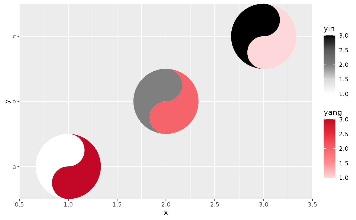
d <- data.frame(x = 1:3, y = c("a", "b", "c"), yin = 1:3, yang = 3:1)
# auto-detects x as continuous and y as discrete
ggplot(d, aes(x, y)) +
geom_taichi(yin = yin, yang = yang) +
remove_padding()
 # explicit override, identical result here
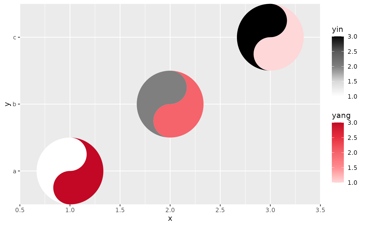
ggplot(d, aes(x, y)) +
geom_taichi(yin = yin, yang = yang) +
remove_padding(x = "c", y = "d")
# explicit override, identical result here
ggplot(d, aes(x, y)) +
geom_taichi(yin = yin, yang = yang) +
remove_padding(x = "c", y = "d")